Results matching “R”

In a comment here, Martin Termouth cited this report from Nature, "One in three scientists confesses to having sinned."

But what are these sins? Here's the relevant table:

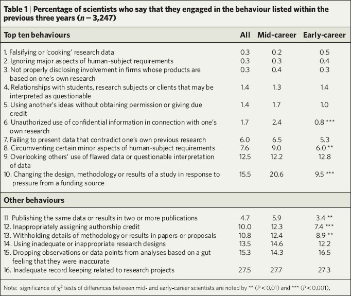
This looks pretty bad, until you realize that the rarest behaviors, which are also the most severe, are at the top of the table. The #1 "sin," admitted-to by 15.5% of the respondents, is "Changing the design, methodology or results of a study in response to pressure from a funding source." But is that a sin at all? For example, I've had NIH submissions where the reviewers made good suggestions about the design or data analysis, and I've changed the plan in my resubmission. This is definitely "pressure"--it's not a good idea to ignore your NIH reviewers--but not improper at all.

From the other direction, as an NSF panelist I've made suggestions for research proposals, with the implication that they better think very hard about alternative designs or analyses if they want to get funding. This all seems proper to me. Of course, I agree that it's improper to change the results of a study in response to pressure. But, changing the design or methodology, that seems OK to me.

Now let's look at the #2 sin, "Overlooking others' use of flawed data or questionable interpretation of data." This is not such an easy ethical call. Blowing the whistle on frauds by others is a noble thing to do, but it's not without cost. My friend Seth Roberts has, a couple times, pointed out cases of scientific fraud (here's one example), and people don't always appreciate it. Payoffs for whistleblowing are low and the costs/risks are high, so I'd be cautious about characterizing "Overlooking other's use of flawed data..." as a scientific "sin."

Now, the #3 sin, "Cirumventing certain minor aspects of human-subjects requirements." I agree that this could be "questionable" behavior. Although I'm not quite sure if "circumventing" is always bad. It's sort of like the difference between "tax evasion" (bad) and "tax avoidance" (OK, at least according to Judge Learned Hand).

Taking out these three behaviors leaves 11.4%, not quite as bad as the "more than a third" reported. (On the other hand, these are just reported behaviors. I bet there's a lot more fraud out there by people who wouldn't admit to it in a survey.)

If you've read this far, here's a free rant for you!

P.S. When you click on a Nature article, a pop-up window appears, from "c1.zedo.com", saying "CONGRATULATIONS! YOU HAVE BEEN CHOSEN TO RECEIVE A FREE GATEWAY LAPTOP . . . CLICK HERE NOW!." Is this tacky, or what? I thought the British were supposed to be tasteful!

Eric Oliver is speaking todayin the American Society and Politics Workshop on "fat politics." Here's the paper and here are some paragraphs from it:

In truth, the only way we are going to “solve” the problem of obesity is to stop making fatness a scapegoat for all our ills. This means that public health officials and doctors need to stop making weight a barometer of health and issuing so many alarmist claims about the obesity epidemic. This also means that the rest of us need to stop judging others and ourselves by our size.

Such a change in perspective, however, may be our greatest challenge. Our body
weight and fatness is a uniquely powerful symbol for us – something we feel we should
be able to control but that often we can’t. As a result, obesity has become akin to a
sacrificial animal, a receptacle for many of our problems. Whether it is our moral
indignation, status anxiety, or just feelings of general powerlessness, we assume we can
get a handle on our lives and social problems by losing weight. If we can only rid
ourselves of this beast (that is, obesity), we believe we will not only be thin, but happy,
healthy, and righteous. Yet, as with any blind rite, such thinking is a delusion and
blaming obesity for our health and social problems is only going to cause us more injury
over the long haul.

So how might we change our attitudes about obesity and fat? As with any change
in perspective, the first place we must begin is in understanding why we think the way we
do. In the case of obesity, we need to understand both why we are gaining weight and,
more importantly, why we are calling this weight gain a disease. In other words, if we
are to change our thinking about fat, we need to recognize the real sources of America’s
obesity epidemic.

Oliver continues:

Monday talk (for general audience):

Mathematical vs. statistical models in social science

Mathematical arguments can give insights into social phenomena but, paradoxically, tend to give qualitative rather than quantitative predictions. In contrast, statistical models, which often look messier, can introduce new insights. We give several examples of interesting, but flawed, mathematical models for examples including political representation, trench warfare, the rationality of voting, and the electoral benefits of moderation. We consider ways in which these models can be improved in these examples. We also discuss more generally why mathematical models might be appealing and why they commonly run into problems.

Tuesday talk (for math/stat majors and other interested parties):

Coalitions, voting power, and political instability

We shall consider two topics involving coalitions and voting. Each topic involves open questions both in mathematics (probability theory) and in political science.
(1) Individuals in a committee or election can increase their voting power by forming coalitions. This behavior yields a prisoner's dilemma, in which a subset of voters can increase their power, while reducing average voting power for the electorate as a whole. This is an unusual form of the prisoner's dilemma in that cooperation is the selfish act that hurts the larger group. The result should be an ever-changing pattern of coalitions, thus implying a potential theoretical explanation for political instability.
(2) In an electoral system with fixed coalition structure (such as the U.S. Electoral College, the United Nations, or the European Union), people in diferent states will have different voting power. We discuss some flawed models for voting power that have been used in the past, and consider the challenges of setting up more reasonable mathematical models involving stochastic processes on trees or networks.

If people want to read anything beforehand, here's some stuff for the first talk:

http://www.stat.columbia.edu/~gelman/research/unpublished/trench.doc
http://www.stat.columbia.edu/~gelman/research/unpublished/rational_final5.pdf
http://www.stat.columbia.edu/~gelman/research/published/chance.pdf

and here's some stuff for the second talk:

http://www.stat.columbia.edu/~gelman/research/published/blocs.pdf
http://www.stat.columbia.edu/~gelman/research/published/STS027.pdf
http://www.stat.columbia.edu/~gelman/research/published/gelmankatzbafumi.pdf

Gary writes about the social science of architecture, after being deeply involved in the design and construction of a new office building. Key quote:

Ultimately the goal of this particular $100M-plus building, and of most buildings built by universities, is not only to create beautiful surroundings but also to increase the amount of knowledge created, disseminated, and preserved (my summary of the purpose of modern research universities). . . . As such, some systematic data collection could have a considerable impact on this field. Do corridors or suites make the faculty and students produce and learn more? Does vertical circulation work as well as horizontal? Should we put faculty in close proximity to others working on the same projects or should we maximize interdisciplinary adjacencies? . . .

From another perspective, and speaking as a consumer rather than a designer of architecture, I'd be interested in a study of the incentives to architects. My completely unscientific impression is that a lot of buildings that were built during the 1960s and 1970s were poorly functional--often too hot or too cold, hard to find the entrances, hard to find your way around the building, and not making good use of the available land. Since then, public buildings have improved. Anyway, I wonder about the incentives for these architects. Do they advance in their career by building interesting but non-functional buildings? What is their incentive to build something that can work well?

Gary's proposal, of taking lots of outcome measurements on building use, could be helpful for the reasons he states (to evaluate architectural plans) but also as a motivation, even as a reminder to builders that these outcomes are relevant goals. (Just as, by analogy, student evaluations put some pressure on teachers and remind us not to forget about the students in our classes.) Feedback is good.

Also, regarding Gary's proposed study of office buildings, you could also make a study of private houses. This gives you a potentially huge N, and also raises issues of public/private priorities (lawns vs. parks, etc.). I've seen a million statistical papers on real estate prices, but little or nothing on outcomes relating to the houses as experienced by the residents..

I went to Radio Shack the other day and bought a telephone answering machine.

Q: Did I want to buy the extended warranty for $5.99? [Students: figure this one out before continuing...]

I can't believe Nixon won. I don't know anybody who voted for him. -- mistakenly attributed to Pauline Kael, 1972

It evidently irritates many liberals to point out that their party gets heavy support from superaffluent "people of fashion'' and does not run very well among "the common people.'' -- Michael Barone, 2005

Both these quotes correspond to political misunderstandings which I thiink can be attributed to a well-known cognitive bias.

First-order and second-order availability biases

Psychologists have studied the "availability bias"--the phenomenon that people tend to overweight their own experiences when making decisions or judging rates or probabilities. I was thinking about this, in regard to political commentators who are trying to understand who's voting for whom in presidential elections.

In this case, we could speak of first-order and second-order availability biases. A national survey of journalists found that about twice as many are Democrats as Republicans. Presumably their friends and acquaintances are also more likely to support the Democrats, and a first-order availability bias would lead a journalist to overestimate the Democrats' support in the population--as in the above quote that had been attributed to Pauline Kael.

However, political journalists are well aware of the latest polls and election forecasts and are unlikely to make such an elementary mistake. However, they can well make the second-order error of assuming that the correlations they see of income and voting are representative of the population. Weaver et al. (2003) found that 90% of journalists are college graduates and have moderately high incomes--so it is natural for them to think that they and their friends represent Democrats as a whole. Michael Barone, for example, although no liberal himself, probably knows many affluent liberal Democrats and then, from a second-order availability bias, imputes an incorrect correlation of income and Democratic voting to the general population. (Just to be clear on this point: richer voters tend to support the Republicans. Barone, should know better but was, I believe, faked out by a second-order availability bias. These cognitive biases can fake out the best of us--they come from inside our head and avoid our usual barriers of skepticism.)

When considering income and voting, the second-order availability bias is exacerbated by geographic patterns

Another form of availability bias is that the centers of national journalistic activity are relatively rich states including New York, California, Maryland, and Virginia. Once again, the journalists--and, for that matter, academics--avoid the first-order availability bias: unlike "Pauline Kael" (in the mistakenly-attributed quote), they are not surprised that the country as a whole votes differently from the residents of big cities. But they make the second-order error of too quickly generalizing from the correlations in their states. It turns out (as we show in our forthcoming paper) that richer counties tend to support the Democrats within the "media center'' states but not, in general, elsewhere. And richer voters support the Republicans just about everywhere, but this pattern is much weaker--and thus easier to miss--within these states.

Much has been written in the national press about the perils of ignoring "red America'' but these second-order availability biases have done just that, in a more subtle way.

Tyler Cowen links to Matt Yglesias linking to a quote from Frans De Waal, who's writing about a method of evaluating conversations using low-frequency voice patterns. Anyway, here's the relevant paragraph from De Waal:

The same spectral analysis has been applied to televised debates between U.S. presidential candidates. In all eight elections between 1960 and 2000 the popular vote matched the voice analysis: the majority of people voted for the candidate who held his own timbre rather than the one who adjusted.

But the elections of 1960, 1968, 1976, and 2000 were essentially tied. You get no credit for predicting the "winner" in any of these, any more than you would get credit for correctly predicting the outcome of a coin flip. (This is a point I made back in 1992 in my review of a book on forecasting elections.)

Anyway, I'm not trying to criticize (or evaluate in any way) what De Waal is doing--let's just not ovestate the evidence here.

Jens Hainmueller refers to a paper by David Lee, "Randomized experiments from non-random selection in U.S. House elections." In the paper, Lee uses a regression discontinuity analysis to compare election outcomes in districts that, two years earlier, were either barely won by Democrats or barely won by Republicans. The difference between these districts in the next election can be identified as the causal effect of the incumbent party--that is, the difference it makes, having a Democrat or a Republican running, in otherwise nearly-identical districts.

Lee's analysis is fine, and he has a nice picture on page 33 of his paper showing his model and how his estimate compares to that of Gelman and King (1990). However, he is wrong to label what he is estimating as "the electoral advantage to incumbency." He is more precise in Section 3.5 and Appendix B of his paper, when he refers to his estimate of "the incumbent party advantage." The difference is, as Lee makes clear in his paper, that in a hypothetical world in which incumbency itself were worth nothing--in which a Democrat in an open seat would run as well as a Democrat who is an incumbent--you could still have a nonzero incumbent party advantage, if voters preferred to stick with the same party they had before. So I agree with the message of Lee, that both these things--the incumbent party advantage and the incumbency advantage--are interesting. As Gary and I discuss on page 1153 in our 1990 paper, yet another quantity of interest is the personal incumbency advantage, a quantity that has also been studied by Cox, Katz, Ansolabehere, and others.

On a related point, I think Lee is misleading when he says (on page 28) that "the regression discontinuity estimates cannot be recovered from a Gelman-King type analysis." I mean, yes, we use a linear model on vote proportions, and he has a model of probabilities. But we do have an incumbent party effect--it is the coefficient of the incumbent party indicator P_2 in our model--so we did in fact estimate this (within the context of a linear model).

One other, more technical issue: there is a lot of information in the actual vote shares received by the candidates, which is why political scientists typically model these directly. Modeling vote shares gives you the efficiency to get separate estimates for each election year and thus study time trends. I understand the appeal of simply looking at winning and losing, but there is much to be learned by studying vote shares.

In summary, I like Lee's paper, and it's good to see connections between different social sciences. For the particular example of incumbency advantage, I'd have more trust in simple regression estimators, separating the effects of incumbent party (P_i) and incumbency (I_i) as discussed in our 1990 paper and in Lee's Appendix B. Or, to go in new directions, using the Bayesian method of Gelman and Huang (2006, to appear). But it can't hurt to have new methods, and for other problems where the linear model doesn't work so well, I could see Lee's method providing a real advance.

Statisticians continue to be in demand, especially those who are interested in social science and policy applications. From Susan Paddock at RAND:

Today I came across a paper in my files, "On a limiting process which asymptotically produces f^{-2} spectral density" from 1962 by Hirotugu Akaike (most famous for his information criterion). The paper has a great opening paragraph:

In the recent papers in which the results of the spectral analyses of roughnesses of runways or roadways are reported, the power spectral densities of approximately the form f^{-2} (f: frequency) are often treated. This fact directed the present author to the investigation of the limiting process which will provide the f^{-2} form under fairly general assumptions. In this paper a very simple model is given which explains a way how the f^{-2} form is obtained asymptotically. Our fundamental model is that the stochastic process, which might be considered to represent the roughness of the runway, is obtained by alternative repetitions of roughening and smoothing. We can easily get the limiting form of the spectrum for this model. Further, by taking into account the physical meaning of roughening and smoothing we can formulate the conditions under which this general result assures that the f^{-2} form will eventually take place.

It's a cool paper, less than 5 pages long. Something about this reminds me of Mandelbrot's early papers on taxonomy and Pareto distributions, written about the same time.

In a recent article in the New York Review of Books (see also here), Freeman Dyson writes,

Great scientists come in two varieties, which Isaiah Berlin, quoting the seventh-century-BC poet Archilochus, called foxes and hedgehogs. Foxes know many tricks, hedgehogs only one. Foxes are interested in everything, and move easily from one problem to another. Hedgehogs are interested only in a few problems which they consider fundamental, and stick with the same problems for years or decades. Most of the great discoveries are made by hedgehogs, most of the little discoveries by foxes. Science needs both hedgehogs and foxes for its healthy growth, hedgehogs to dig deep into the nature of things, foxes to explore the complicated details of our marvelous universe. Albert Einstein was a hedgehog; Richard Feynman was a fox.

This got me thinking about statisicians. I think we're almost all foxes! The leading stasticians over the years all seem to have worked on lots of problems. Even when they have, hedghehog-like, developed systematic ideas over the years, these have been developed in a series of applications. It seems to be part of the modern ethos of statistics, that the expected path to discovery is through the dirt of applications.

I wonder if the profusion of foxes is related to statistics's position, compared to, say, physics, as a less "mature" science. In physics and mathematics, important problems can be easy to formulate but (a) extremely difficult to solve and (b) difficult to understand the current research on the problem. It takes a hedgehog-like focus just to get close enough to the research frontier that you can consider trying to solve open problems. In contrast, in statistics, very little background is needed, not just to formulate open problems but also to acquire many of the tools needed to study them. I'm thinking here of problems such as how to include large numbers of interactions in a model. Much of the progress made by statisticians and computer scientists on this problem has been made in the context of particular applications.

Going through some great names of the past:

Don Rubin published an article in 2002 on "The ethics of consulting for the tobacco industry." Here's the article, and here's the abstract:

This article describes how and why I [Rubin] became involved in consulting for the tobacco industry. I briey discuss the four relatively distinct statistical topics that were the primary focus of my work, all of which have been central to my published academic research for over three decades: missing data; causal inference; adjustment for covariates in observational studies; and meta-analysis. To me [Rubin], it is entirely appropriate to present the application of this academic work in a legal setting.

My thoughts:

I respect what Don is saying here--I don't think he'd do this sort of consulting without thinking it through. At the same time, I think there are a couple of complications not mentioned in his article.

Paul Gustafson and Sander Greenland have a preprint entitled, "The Performance of Random Coefficient Regression in Accounting for Residual Confounding." From their paper:

The problem studied in detail by Greenland (2000) involves a case-control study of diet, food constituents, and breast cancer. The exposure variables are intakes of 35 food constituents (nutrients and suspected carcinogens), each of which is computed from responses to an 87-item dietary questionnaire. An analysis based on the 35 food constituents alone assumes that the 87 diet items have no effect beyond that mediated through the food constituents. Greenland (2000) comments that this is a strong and untenable assumption. As an alternative he included both the food constituents and the diet items in a logistic regression model for the case-control status, while acknowledging that this model is formally nonidentified since each food constituent variable is a linear combination of the diet variables. To mitigate the lack of identifiability, a prior distribution is assigned to the regression coefficients for the diet variables, i.e., random coefficient regression is used. The prior distribution has mean zero with small variance, chosen to represent the belief that these coefficients are likely to be quite small typically, as they represent `residual confounding’ effects of diet beyond those represented by the food constituents. Greenland argued that, however questionable this prior may be, it is surely better than the standard frequentist analyis of such data, which omits the diet variables entirely – equivalent to using the random-coefficient model with a prior distribution that has variance (as well as mean) zero.

I have long felt that hierarchical modeling is the way to go in regression with large numbers of related predictors, but I was not familiar with the Greenland (2000) paper. Section 5.2.3 of my 2004 Jasa paper on parameterization and Bayesian modeling presents a similar idea, but I've never actually carried it out in a real application. So I'd be interested in seeing more about Greenland's example.

P.S. I like the following quote in the abstract of Greenland's paper:

The argument invokes an antiparsimony principle attributed to L. J. Savage, which is that models should be rich enough to reflect the complexity of the relations under study. It also invokes the countervailing principle that you cannot estimate anything if you try to estimate everything (often used to justify parsimony). Regression with random coefficients offers a rational compromise . . .

This accords with my views on parsimony and inference (see also here and here).

P.P.S. On a technical level, I'm disturbed that Gustafson and Greenland use inverse-gamma prior distributions for their variance parameters. I think this is too restrictive as a parametric family. Ironically, the family of prior distributions I've proposed has the same mathematical form as the multiplicative models that can be used for varying coefficients.

In a recent article in the New York Review of Books, Freeman Dyson quotes Richard Feyman:

No problem is too small or too trivial if we really do something about it.

This reminds me of the saying, "God is in every leaf of every tree," which I think applies to statistics in that, whenever I work on any serious problem in a serious way, I find myself quickly thrust to the boundaries of what existing statistical methods can do. Which is good news for statistical researchers, in that we can just try to work on interesting problems and the new theory/methods will be motivated as needed. I could give a zillion examples of times when I've thought, hey, a simple logistic regression (or whatever) will do the trick, and before I know it, I realize that nothing off-the-shelf will work. Not that I can always come up with a clean solution (see here for something pretty messy). But that's the point--doing even a simple problem right is just about never simple. Even with our work on serial dilution assays, which is I think the cleanest thing I've ever done, it took us about 2 years to get the model set up correctly.

As the saying goes, anything worth doing is worth doing shittily.

Alex Tabarrok writes, regarding the example in Section 3 of this paper,

Another nice illustration of the importance of weighting comes from high-stakes schemes that reward schools for improving test scores. North Carolina, for example, gives significant monetary awards to schools that raise their grades the most over the year. The smallest decile of schools has been awarded the highest-honors (top-25 in the state) 27% of the time while schools in the largest decile have received that honor only about 1% of the time. Students (and parents) are naturally led to believe that small schools are better. But just as with the cancer data, the worst schools also come from the smallest decile. The reason, of course, is the same as with the cancer data small changes in incoming student cohorts make the variance of the score changes much larger at the smaller schools. There are some nice graphs and discussion in

Kane, T. and D. O. Staiger. 2002. The Promise and Pitfalls of Using Imprecise School Accountability Measures. Journal of Economic Perspectives 16 (4):91-114.

It's scary to think of policies being implemented based on the fallacy of looking at the highest-ranking cases and ignoring sample size. But most of my students every year get the cancer-rate example wrong--that's one reason it's a good example!--so I guess it's not a surprise that policymakers can make the mistake too. And even though people point out the error, it can be hard to get the message out. (For example, Kane and Staiger hadn't head of my paper with Phil Price on the topic, and until recently, I hadn't heard of Kane and Staiger's paper either.)

I just came back from a talk by Jere Behrman on "What Determines Adult Cognitive Skills? Impacts of Pre-School, School-Years and Post-School Experiences in Guatemala." Here's the paper.

It was all interesting, but what confused me here, as in other talks of this type, was the interpretation of regressions controlling for several variables that are sequential in time. This particular example was a longitudinal study of about 1500 people, looking at adult cognitive outcomes and including, as predicotrs, measures of health at age 6, years of schooling, and work after school was over. It's tricky to interpret the coefficient of pre-school health in this regression as a "treatment effect" since it can affect the other predictors. People at the seminar were talking along the lines of "causal pathways" but this always confuses me too. A simple response is to follow the basic advice of not controlling for post-treatment outcomes, but doing such an analysis wouldn't address some of the questions the researchers were trying to study here.

So I'm left simply confused. I'm not trying to be critical of this paper, since I'm not really offering an alternative. But I'm not quite sure how to interpret all these regression coefficients. (Even setting aside the issues involving instrumental variables, which are used in this study also.) I'm just a little stuck here.

Paul Del Piero, a student at Pomona College, did a study of four redistricting plans in California. He uses uniform partisan swing (which can be viewed as an approximation to the method used by the Judgeit program developed by Gary King and myself) to estimate seats-votes curves. Here's his paper, here are the appendices for the paper, and here's the abstract.

I also have one comment of my own, which I'll give after Paul's abstract:

Could it make sense for the Republicans to support geographically-localized policies that help the poor and geographically-diffuse policies that help the rich?

Brett Pelham (whose research on names and life choices is discussed here and here--based on the work of Pelham and his collaborators, we crudely estimate that about 1% of people in the U.S. choose a career based on their first name) wrote a quick email in response.

Jouni pointed me to this page, at Harvard's Bok Center for Teaching and Learning, on teaching by having students work in groups. As Jouni says, and I agree,

It seems to me that from the "liberal" (in the U.S. politics) perspective, man [humans] used to be the "rational animal" but is now the "irrational computer," and this worries me a bit.

The rational animal

For an example of the first view, here's a quote I just googled::

"We believed . . . that man was a rational animal, endowed by nature with rights, and with an innate sense of justice; and that he could be restrained from wrong and protected in right, by moderate powers, confided to persons of his own choice, and held to their duties by dependence on his own will." -- Thomas Jefferson, 1823

The idea being that our rationality is what separates us from the beasts, either individually (as in the Jefferson quote) or through collective action, as in Locke and Hobbes. If the comparison point is animals, then our rationality is a real plus!

The irrational computer

Nowadays, though, it seems almost the opposite, that people are viewed as irrational computers. To put it another way, if the comparison point is a computer, then what makes us special is not our rationality but our emotions.

I was thinking about this when reading in n+1 magazine the review by Megan Falvey of the book "Freakonomics."

Our description of the rational self supports the real-world conditions under which some futures seem more attainable than others. It coaxes us into wholehearted, personally felt participation with capitalist regulation. Levitt's calculating individual is the ideal subject of contemporary neoliberal economic reform, in particular the expansion of the market into all possible areas of life.

The idea seems to be that "the description of the rational self" excludes warmer aspects of human nature. That I'll definitely believe. But I still think rationality is a good thing--perhaps my bias as a scientist.

Decoupling rationality and selfishness

Rationality can serve other-directed as well as selfish goals. Yes, I can rationally try to get the best deal on a new TV, but the Red Cross can also use rationality (for example, in the form of mathematical optimization) to deliver help to as many people as possible. Or Novartis can use rationality (in the form of up-to-date biostatistical methods) to increase the chance of developing an effective drug--this can serve both selfish and unselfish purposes.

The decoupling of rationality and selfishness is a point we made here, in the context of considering voting as a rational way to attempt to improve the well-being of others as well as oneself.

To get back to Falveys' book review: I'm not attempting to address the details of her disagreements with Levitt and Dubner, just to express my distress that she sees rationality to be a problem. Considering the alternatives, I think rationality is pretty good. But it is useful to think about the goals to which the rationality is directed.

From Chance News, submitted to Chance News by Bill Peterson, based on a posting from Joy Jordan to the Isolated Statisticians e-mail list:

Exploiting the gender gap New York Times, 5 September, 2005, A21 Warren Farrell

Farrell is the author of Why Men Earn More: The Startling Truth Behind the Pay Gap -- and What Women Can Do About It (AMACOM, 2004)

This article was published for Labor Day, and it opens by citing a demoralizing, often-heard statistic: women still earn only 76 cents for each dollar paid to their male counterparts in the workplace. Farrell maintains that such comparisons ignore important lurking variables. He claims to have identified twenty-five tradeoffs involving job vs. lifestyle choices, all of which men tend to resolve in favor of higher pay, while women tend to seek better quality of life.

Here are some the factors discussed in the article. Men more readily accept jobs with longer hours, and Farrell reports that people who work 44 hours per work earn twice as much as people who work 34 hours per week. Similarly, he finds that men are more willing to relocate or travel, to work in higher risk environments, and to enter technical fields where jobs may involve less personal interaction. Each of these choices is associated with higher pay.

Even head-to-head comparisons of men and women working in the “same job” can be tricky. Farrell observes, for example, that Bureau of Labor Statistics data consider all medical doctors together. But men opt more often for surgery or other higher paid specialties, while women more often choose general practice.

As indicated by the subtitle of his book, however, Farrell intends to provide some positive news for women. He claims that in settings where women and men match on his 25 variables, the women actually earn more than men. He also identifies a number of specific fields where women do better. One of these is statistics(!), where he reports that women enjoy a 35 percent advantage in earnings.

I haven't read the book so can't comment on the analysis, but it seems like a great discusison topic for class.

Jim Hodges, Yue Cui, Daniel Sargent, and Brad Carlin completed their paper on "smoothed Anova". The abstract begins: "We present an approach to smoothing balanced, single-term analysis of variance (ANOVA) that emphasizes smoothing interactions, the premise being that for a dependent variable on the right scale, interactions are often absent or small. . . ."

The topic is hugely important, I believe (see also here): especially in observational studies, regression models work because they can handle multiple inputs (for example, see Michael Stastny's quick discussion here). Once we have multiple inputs, you gotta look at interactions, which quickly leads to a combinatorical explosion, the usual "solution" to which is to ignore high-level interactions. But in some problems--including many decision analyses and many research studies in psychology--interactions are what we really care about. (Here's an example from our own work where we would have liked to include more interactions than we actually did.)

Anyway, I think this is one of the major unsolved problems in statistics. It can be attacked in several ways, including regression/Anova (that's where Hodges et al. and I are working), neural nets, nonparametric models, etc etc. My best published method so far of handling high-level interactions isn't so great, and I think that Hodges et al. are doing interesting stuff.

I hope lots of people read the article, try out the methods presented there, and take the ideas even further.

I don't really want to go on and on about this, but since it's a current research topic of ours . . .

I'm trying to integrate class-participation activities into the Applied Regression and Multilevel Modeling course I'm teaching this semester. We have a whole bunch of these activities for introductory statistics (in my intro class I have at least one demo and one other activity per lecture) but I've never before tried to consistently use them for a more advanced class.

I'll tell you how things have been going so far and then update occasionally.

The first 2 weeks: what they need to learn

The first several weeks of the class are a review of classical (non-multilevel) regression, with a focus on understanding the model, particularly the deterministic part (that is, y=a+bx, with less of a focus on the distirbution of epsilon). This is also a time for the students to get familiar with R, which they'll have to use more of when working with more complicated models--especially when trying to use inferences beyond simply looking at parameter estimates and standard errors. The first two homework assignments involve fitting simple regressions in R, graphing the data and the fitted regression lines, and building a multiple regression to fit Hamermesh's beauty and teaching evaluations data. Jouni, as T.A., has to spend a lot of time helping students get started with R. The main mathematical difficulties are learning and understanding linear and logarithmic transformations.

The first 2 weeks: in the classroom

Lecture 1 starts with some motivating examples, including roaches, rodents, and red/blue states. I stop and give the students a few minutes to work in pairs to come up with explanations for the patterns of income and voting within and between states. I describe the roach study and the rodent study and then give the students a minute to discuss in pairs to see if they can figure out the key difference between the two studies. (The difference is that the roach study has the goal of estimating a treatment effect--integrated pest management compared to usual practice--and the rodent study is descriptive--to understand the differences between rodent levels in apartments occupied by whites, blacks, hispanics, and others. We'll get back to causal inference in a few weeks.) I yammer on a bit about the skills they'll learn by the time the course is over, and how I expect them to teach themselves these skills. Analogies between statistics and child care, sports, and policy analysis. Cautionary examples of Dan Marino and Cal Ripken. The beauty and teaching evaluations example. I give the equation of the regression line, the students have to work in pairs to draw it. Use the computer to fit some regressions in R and plot the data and fitted regression lines. (No residual plot for now, no q-q plot: we're focusing on the important things first.)

Lecture 2 starts with the cancer-rate example. I hand out Figure 2.7 from BDA and give the students a few minutes to work in pairs to come up with explanations for why the 10% of counties with highest kidney-cancer deaths are mostly in the middle of the country. I write various explanations on the blackboard and then hand out Figure 2.8. We discuss: this is a motivator for multilevel models. I was going to bring up the example of the test with 1 or 100 questions but forgot to mention it--maybe I'll do it in class in a few weeks. I then give them the regression of earnings (in 1993) on height (in inches): y = -61000 + 1300*height + error, with residual sd of 19000. In pairs, they must draw the line and hypothetical data that would lead to this estimated regression. This is a toughie--the students have to realize that heights are mostly between 60 and 75 inches, and that the data must be skewed to all fit above the y=0 line. We talk transformations for a bit--some more activities in pairs (for example, what's the equation of the regression line if we first normalize x by subtracting its mean and dividing by its sd). Discussion of appropriate scale of the measurements and how much to round off. Comparisons of men to women: adding sex into the regression model. In pairs: what's the difference in earnings between the avg man and the avg woman (it's not the coef for sex, since the two sexes differ in height). Why it's better to create a variable called "male" than one called "sex."

Lecture 3 starts with answering questions. What are outliers and should we care about them? (My answer: outliers are overrated as a topic of interest.) Why is it helpful to standardize input variables before including interactions? Long discussion using the earnings, height, and sex example. Standardize earnings by subtracting mean and dividing by 2*sd. Standardize sex by recoding as male=1/2, female=-1/2. Lots of working in pairs drawing regression lines and figuring out regression slopes. Understanding coefficients of main effects and interactions. Categorized predictors, for example modeling age as continuous, with quadratic term, using discrete categories. Start talking about the logarithm. The amoebas example--at time 1, there is 1 amoeba; at time 2, 2 amoebas, at time 3, 4 amoebas; etc. In pairs: give the equation of #amoebas as a function of time. Then give the linear relation on the log scale. (I should have had this example starting at time 0. Having to subtract time=1 is a distraction that the students didn't need.) Graph of world population vs. time since year 1, graph on log scale. Interpreting exponential growth as a certain percentage per year, per 100 years (in pairs again).

Lecture 4: all about logarithms. On the blackboard I give the equation for a cube's volume V as a function of its length L. Then also log V = 3 log L. Then, in pairs, they have to figure out the corresponding formulas for surface area S as a function of volume. It's not so easy for students who haven't used the log in awhile. Then we discuss the example of metabolic rate and body mass of animals. We then go to interpreting log regression models. Log earnings vs. height. Log earnings vs. log height. Interpreting log-regression coefficients as multiplicative factors (if the coef is 0.20, then a 1-unit difference in x corresponds to an approximate 20% difference in y). Interpreting log-log coefficients as elasticities (if the coef is 0.6, then a 1% increase in x corresponds to an approximate 0.6% increase in y). All these are special cases of transformations. Also discuss indicator variables, combinations of inputs, and model building. How to interpret statistical significance of regression coefficients. We did some more activities in pairs but I can't quite remember what they were.

How do I have time to cover the material?

People have often told me that they'd like to do group activities but they can't spare the class time. I disagree with that line of thinking. My impression is that students learn by practicing. A lecture can be good because it gives students a template for their own analyses, or because it motivates students to learn the material (for example, by demonstrating intersting applications or counterintuitive results), or by giving students tips on how to navigate the material (e.g., telling them what sections in the book are important and what they can skip, helping them prepare for homework and exams, etc.). The lecture room also can be a great way to answer questions, since when one student has a question, others often have similar questions, and the feedback is helpful as the class continues.

But I don't see the gain in "covering" material. I don't need to do everything in lecture. It's in the book, and they're only going to learn it if its in the homeworks and exams anyway. The class-participation activities allow the students to confront their problem-solving difficulties in an open setting, where I can give them immediate feedback and help them develop their skills. And having them work in pairs keeps all of them (well, most of them) focused during my 9-10:30am class.

Summary (so far)

This has been pretty exciting so far. We'll see how it works for the whole semester. At this point, I don't even think I'm capable of doing straight lectures, so it's good that the activities are working. But maybe . . . maybe . . . this could transform the teaching of statistics! It's a hope (or distant goal).

Here's the revised version of our paper on why and how it's rational to vote, and here's the abstract:

.For voters with "social" preferences, the expected utility of voting is approximately independent of the size of the electorate, suggesting that rational voter turnouts can be substantial even in large elections. Less important elections are predicted to have lower turnout, but a feedback mechanism keeps turnout at a reasonable level under a wide range of conditions. The main contributions of this paper are: (1) to show how, for an individual with both selfish and social preferences, the social preferences will dominate and make it rational for a typical person to vote even in large elections; (2) to show that rational socially-motivated voting has a feedback mechanism that stabilizes turnout at reasonable levels (e.g., 50% of the electorate); (3) to link the rational social-utility model of voter turnout with survey findings on socially-motivated vote choice.

What's cool about the social-benefit model is it not only explains why it is rational to vote (and to participate in politics in other ways, such as by making small contributions to political campaigns) but also makes it clear that, to the extent it is rational to vote, it is rational for the choice of whom to vote for to depend on social rather than selfish preferences.

For more on this and related topics, see these earlier blog entries here, here, and here. And some stuff here on voting and social networks.

My entry on the boxer and the wrestler sparked some interesting discussion here and here. In order to understand the distinction between randomness and uncertainty in a probability distribution, one has to embed that probabability into a larger structure with potentially more information. As Aki Vehtari pointed out, Tony O'Hagan made this point in a nice article published last year.

Dempster-Shafer not a solution. Neither is robust Bayes

Anyway, one of the other comments on my post alluded to belief functions (Dempster and Shafer's theory of upper and lower probabilities) as a solution to the boxer/wrestler paradox. Actually, though, the boxer/wrestler thing was part of something that Augustine Kong and I came up with 15 years ago as a counterexample, or paradox, for Bayesian inference, robust Bayes, and also belief functions. For this particular example, the answer given by belief functions doesn't make much sense.

Here's my recent paper on the topic, and here's the abstract to the paper:

Bayesian inference requires all unknowns to be represented by probability distributions, which awkwardly implies that the probability of an event for which we are completely ignorant (e.g., that the world's greatest boxer would defeat the world's greatest wrestler) must be assigned a particular numerical value such as 1/2, as if it were known as precisely as the probability of a truly random event (e.g., a coin flip).

Robust Bayes and belief functions are two methods that have been proposed to distinguish ignorance and randomness. In robust Bayes, a parameter can be restricted to a range, but without a prior distribution, yielding a range of potential posterior inferences. In belief functions (also known as the Dempster-Shafer theory), probability mass can be assigned to subsets of parameter space, so that randomness is represented by the probability distribution and uncertainty is represented by large subsets, within which the model does not attempt to assign probabilities.

Through a simple example involving a coin flip and a boxing/wrestling match, we illustrate difficulties with pure Bayes, robust Bayes, and belief functions. In short: pure Bayes does not distinguish ignorance and randomness; robust Bayes allows ignorance to spread too broadly, and belief functions inappropriately collapse to simple Bayesian models.

Mark Liberman at Language Log has traced the pirate's "Rrrrr" to a 1950 movie version of Treasure Island. Which reminded me of something. I read Treasure Island a few years ago and was just delighted and amazed by its readability. That plot really moved. Really un-put-downable. (Unfortunately its ending is weak--things get wrapped up a bit too quickly--but otherwise I'd say the book is perfect.) I was also amused that it had all the cliches of the pirate genre--X marks the spot and all that. But of course they weren't cliches back then--or were they?? I seem to recall reading somewhere that much of Treasure Island was ripped off from a book from the 1820s or so. (I can't remember the details.) This disturbed me, but then I decided that novels back then were like movies and TV today--it was all about doing a good job, not about originality. I mean, nobody criticizes Martin Scorsese or Steven Spielberg etc. of ripping off old movies--that's just beside the point.

On a related topic, I found Dr. Jekyll and Mr. Hyde also to be incredibly readable, and also very suspenseful. Yes, I knew that the Dr. and the Mr. were the same person, but there was a lot of suspense about what would happen next. This was also an interesting book because I did not find its individual sentences to be well-written--they were foggy, much like the London weather that pervades the book--but on the whole the paragraphs whipped by. In contrast, Moby Dick was just full of sparkling sentences, yet each page was a struggle to read.

In tomorrow's Applied Micro seminar, Regina Almeyda Duran speaks on "Proximate Literacy, Inter and Intrahousehold Externalities and Child Health Outcomes: Evidence from India." Here's the abstract:

In the course of studying social and political polarization, I have been thinking about the perceptions of political polarization over the past few decades. In the 1970s, there was much worrying about the decline of political parties, and a general concern that voters were deciding based on slick advertising and personality-based campaigns rather than on firmer grounds such as party affiliation. Since 2000, many political scientists, sociologists, and commentators have been disturbed by increasing political polarization (the differences between so-called red and blue America, and so forth), and a general concern that Democrats and Republicans can't communicate with each other.

The funny thing is, the commentators were concerned about declining party ID in the 1970s and increased party alignment in the 2000s. Shouldn't one of these have made them happy? Well, there are a lot of ways of looking at this, but one perspective is that most of the scholars and commentators have been Democrats. In the 1970s, most voters were Democrats, but the Republicans were doing pretty well in Presidential elections. It would be natural for a scholar to think: if only voters were sensible and followed their party ID, all would go well. . . . Contrariwise, in the 2000s, the voters are split between the parties, with more identified as conservative than as liberal--but they agree with the Democrats on many specific issues, especially economic issues. Thus, it's natural for a commentator to feel that if only the voters were following issues, rather than the liberal/conservative label, all would go well. . . .

Not that I'm saying there should be no cause for concern. As far as I can tell from books I've read, parties in the 1960s and earlier had a large local component, and voting by party involved a long chain of personal connections. Whereas voting by ideology now, whether liberal or conservative, is often more abstract and media-driven. So I think that it's possible to argue that parties then were beneficial in a way that ideologies now are not. All the same, it's interesting to see how these trends are perceived.

The following arrived in the email yesterday:

Seth Roberts is guest-blogging at Freakanomics with lots of interesting hypotheses about low-budget science, or what might be called "distributed scientific investigation" (by analogy to "distributed computing").

One of the paradoxes of Seth's self-experimentation research is that it seems so easy, but it clearly isn't, as one can readily see by realizing how few scientific findings have been obtained this way. Reading Seth's article in Behavioral and Brain Sciences gave me a sense of how difficult these self-experiments were. They took a lot of time (lots of things were tried), required discipline (e.g., standing 8 hours a day and setting up elaborate lighting systems in the sleep experiments) and many many measurements, and were much helped by a foundation of a deep understanding of the literature in psychology, nutrition, etc.

Also, for those interested in further details of Seth's diet, I'll cut-and-paste something from his blog entry.

Seth writes:

I read a couple of psychology papers recently and was impressed by their thoroughness. Each of these papers (one by Pelham, Mirenberg, and Jones, and one by Roberts) had 10 separate studies covering different aspects of their claims. The standard in applied statistics seems much lower: what's expected is that we do one good data analysis, along with explorations of what might have happened had the data been analyzed differently, assessment of the importance of assumptions, and so on.

Standards are lower in applied statistics

The difference, I think, is that in a statistics paper--even an applied statistics paper--the goal is to study or demonstrate a method rather than to make a convincing scientific case about the application under consideration. I mean, the scientific claims being presented should be plausible, but the standards of evidence seem quite a bit lower than in psychology.

What about other fields? Biology and medicine, oddly enough, seem more like statistics than psychology in their "convincingness" standards. In these fields, it seems common for findings to be reversed on later consideration, and typically a research paper will present the result of just one study. (In medicine, it is common to have review articles that summarize 40 or more studies in an area, and it seems accepted that individual studies are not supposed to be convincing in themselves.)

Political science, economics, and sociology seem somewhere in between. Research papers in these fields will sometimes, but not always, include multiple studies, but there is also often a requirement for a theoretical argument of some sort. It's not enough to show that something happened, you also have to explain how it fits in (or refutes) some theoretical model.

The paradox of importance

Getting back to statistical research, one thing I've noticed is that the most elaborate research can be done on relatively unimportant problems. If there is a hurry to solve some important problem, then we'll use the quickest methods at hand--we don't have the time to waste on developing fancy methods. But if it's something that nobody cares about . . . well, then we can put in the effort to really do a good job! In the long run, these new methods we develop can become the quick methods for the important problems of the future, but meanwhile we often see cutting-edge applied statistical research on problems that are of little urgency.

Matthew Kahn asks, "Why are there so few economists in elected office?" (link from Arnold Kling). He states that 45% of Congressmembers are lawyers (which seems a bit much, I must say!) but only some small number of economists (Matthew names two).

I was curious about this so I looked up some statistics--not on Congress but on the workforce. According to the 1001 Statistical Abstract of the United States (within arms reach of my computer, of course!), there were 139,000 economists employed in the United States, which reprsented 0.1% of the employed population. 1% of 535 is about 1/2, so with at least two economists in Congress, the profession is hardly unrepresented.

Serge Galam of the Laboratoire des Milieux Desordonnees et Heterogenes (the social sciences just sound cooler when they're in French) is speaking here on "Contrarian deterministic effects on opinion dynamics: "the hung elections scenario'". The paper is here.

I'm skeptical of physicists doing social science, but on the other hand, Galam's paper seems somewhat related to some (much simpler) work of mine on coalition-formation as a potential explanation for political instability.

Galam's talk is Wed 14 Sept in 1219 International Affairs Building.

Zhiqiang Tan recently wrote two papers on the theory of causal inference: see here and here. Here are the abstracts:

Scott de Marchi writes, regarding the "blessing of dimensionality":

One of my students forwarded your blog, and I think you've got it wrong on this topic. More data does not always help and this has been shown in numerous applications -- thus the huge lit on the topic. Analytically, the reason is simple. Just for an example, assume your loss function is MSE; then, the uniquely best estimator is E(Y | x) -- i.e., the conditional mean of Y at each point X. The reason one cannot do this in practice is that as the size of your parameter space increases, you never have enough data to span the space. Even if you change the above to a neighborhood around each x, the volume of this hypercube gets really, really ugly for any value of the neighborhood parameter. The only way out of of this is to make arbitrary restrictions on functional form, etc. or derive a feature space (thus "tossing out" data, in a sense).

As I said, there's a huge number of applications where more is not better.
One example if face recognition --increasing granularity or pixel depth
doesn't help. Instead, one must run counter to your intuition and throw
out most of the data by deriving a feature space. And, face recognition
still doesn't work all that well, despite decades of research.

There's a number of other issues -- in your comments on 3 "good" i.v.'s
and 197 "bad" ones, you have to take the issue of overfitting much more
seriously than you do.

My reply: Ultimately, it comes down to the model. If the model is appropriate, then Bayesian inference should deal appropriately with the extra information. After all, discarding most of the information is itself a particular model, and one should be able to do better with shrinkage.

That said, the off-the-shelf models we use to analyze data can indeed choke when you throw too many variables at them. Least-squares is notorious that way, but even hierarchical Bayes isn't so great when the large number of parameters have structure. I think that better models for interactions are out there for us to find (see here for some of my struggles; also see the work of Peter Hoff, Mark Handcock, and Adrian Raftery in sociology, or Yingnian Wu in image analysis). But they're not all there yet. So, in the short term, yes, more dimensions can entail a struggle.

Regarding the problem with 200 predictors: my point is that I never have 200 unstructured predictors. If I have 200 predictors, there will be some substantive context that will allow me to model them.

Seth Roberts's work on self-experimentation is the subject of the Freakonomics column in this Sunday's New York Times. Regular readers of this blog will recall discussions of Seth's work here and here. Also a related study here.

The publicizing of Seth's work also is an interesting example of information transmission. Seth published a paper in Behavioral and Brain Sciences--a top journal, but not enough to get the work much publicity. I posted a link to it on our blog (circulation 200/day), it was picked up by Alex at Marginal Revolution (circulation 10,000/day) and from there was noticed by a columnist for the New York Times (circulation ~ 2 million/day). But I think the high quality of Seth's article in BBS, with all its experimental data and scientific context, was crucial, in convincing the two levels of gatekeeper--Alex and Stephen--that the work could be taken seriously.

Andy Nathan had a question about ordered predictor variables:

Craig Newmark writes:

Some people think Katrina will be bad for Republicans and for conservatives generally. . . . I disagree. . . . I think Katrina will ultimately redound to the benefit of conservatives. The pointed, effective question that conservatives used to pose: "Do you want the same people that run the Post Office and the DMV and the IRS running [fill in the blank] for you?" will now become "Do you want the same folks--local, state, and/or federal bureaucrats, whoever you prefer to blame--that responded to Katrina doing [fill in the blank] for you?"

This is an interesting point. If true, it suggests there is an inherent "moral hazard" for conservative politicians, in that they have a long-term incentive to perform poorly in order to discredit government performance more generally. (I wouldn't think the moral hazard holds in the short-term, since I'd assume that poor performance in office leads to a greater probability of losing the next election. But for a farseeing conservative who is willing to lose the next election, it seems that this moral hazard exists.

Not that moral hazards, or perverse incentives, in politics, are limited to conservatives. It's also been said that liberal politicians have an incentive to maintain poverty (to continue getting the votes of the disaffected poor), that anti-abortion politicians have an incentive to keep abortion legal, and so forth. I'm not quite sure what to make of this, or how to study it empirically. At some level we just have to assume that politicians are motivated by doing the right thing. But it's a little scary to think that a slow response to a disaster could be considered a plus.

Speaking of trendiness . . . in the Collective Dynamics Group this Friday aft:

Speaker: Matt Salganik Affiliation: Graduate Student, Sociology, Columbia

Title: Experiments on the collective generation of superstar cultural objects

The Baby Names site of Laura Wattenberg (which we mentioned here) also has a blog. Lots of fun stuff; for example see the recent entry on short and long names:

This sounds interesting, and it's highly statistical:

Organizing the world's information (the world is bigger than you think!) Craig Neville-Manning Engineering Director and Senior Research Scientist Google Inc.

Today's applied micro lunch seminar (which unfortunately I won't be able to attend):

When: Tuesday, September 6th 1:10-2:00pm

Where: International Affairs Building, Room 1027

Speaker: Olga Gorbachev (Graduate Student)

Title: "Have Our Lives Become More Unstable? An Investigation of
Individual Volatility of Welfare in the U.S. over
1980-2000."

Abstract:

Has the individual volatility of welfare changed and if so how? What
events led to these changes and what are the implications for public
policy? We examine the evolution of individual volatility of welfare
over 1980-2000 using data from two surveys: Panel Study of Income
Dynamics (PSID) and Consumer Expenditure Survey (CEX). We find that
on average, micro level data follows macro trends. But, when
specific groups are considered, substantial differences are
observed. Older generations, those born between 1915 and 1944,
experienced increasing levels of volatility over 1980-2000 period,
and those born between 1960 and 1974, encountered decreasing
volatility, independent of their educational attainment. Those born
between 1945 and 1959 saw a decrease in volatility only if they had
some college education otherwise, they experienced an increased
volatility. We propose several reasons for the divergence of the
patterns and conclude by estimating social cost to the society and
to individual groups from changes in volatility measured over
1980-2000 period.

Awhile ago I discussed the Flynn effect and Seth Roberts's view that the writing in newspapers and magazines had become more sophisticated in the past 50 years--an idea that was consistent with Steven Johnson's book finding increased complexity in TV shows.

Seth just sent me something interesting along these lines. Seth writes:

I saw this in a NY Times article:

On Dec. 8, 1941, the day after the Japanese attack on Pearl Harbor, Representative Charles A. Eaton, Republican of New Jersey, made his case in the House for why the nation should enter the Second World War.

"Mr. Speaker," his speech began, "yesterday against the roar of Japanese cannon in Hawaii our American people heard a trumpet call; a call to unity; a call to courage; a call to determination once and for all to wipe off of the earth this accursed monster of tyranny and slavery which is casting its black shadow over the hearts and homes of every land."

Last year, Senator Sam Brownback, Republican of Kansas, made the case for war in Iraq this way:

"And if we don't go at Iraq, that our effort in the war on terrorism dwindles down into an intelligence operation," he said. "We go at Iraq and it says to countries that support terrorists, there remain six in the world that are as our definition state sponsors of terrorists, you say to those countries: we are serious about terrorism, we're serious about you not supporting terrorism on your own soil."

The linguist and cultural critic John McWhorter cites these excerpts in his new book, "Doing Our Own Thing: The Degradation of Language and Music and Why We Should, Like, Care" (Gotham Books). They not only are typical of speeches made in Congress on both occasions, he argues, but also provide a vivid illustration of just how much the language of public discourse has deteriorated.

Notice that what Brownback said is considerably more conceptually complex than what Eaton said, even though the number of words is about the same.

On first glance (and with all due respect to my complete ignorance of the field of linguistics), I agree with Seth on this one: in terms of content, Brownback's statement is much more sophisticated than Eaton's, and I don't see this as "deterioration" at all.

Seth continued with:

Something similar: A few days ago I read a talk by Richard Hamming called "You and Your Research" (google the title to find it) in which he notes:

John Tukey almost always dressed very casually. He would go into an important office and it would take a long time before the other fellow realized that this is a first-class man and he had better listen. For a long time John has had to overcome this kind of hostility.

Relatively complex ideas in a relatively casual package (Brownbeck, Tukey) causing negative feelings in listeners (McWhorter, "the other fellow").

Perhaps my self-experimentation suffers from a similar problem: How dare he measure his own weight! Or his own mood. It's too casual! This analogy suggests history is on the side of self-experimentation. Business dress, like the speeches of congressmen, has become more casual.

Interesting thoughts. I assume this is the same John McWhorter who contributes to the cool Language Log website. I wonder what McWhorter think of Seth's comments on the complexity of public statements.

P.S. Mark Liberman of Language Log has a long and interesting response here (for some reason, I can't get these things to show in Trackback). Here's what I have to say in response to his comments:

Regarding the particular issue in my posting, I think that Seth was responding to the NYtimes article referrong to how "The language of public discourse has deteriorated." Seth is arguing that, if content increases while style becomes simpler--well, that's not deterioration at all, but rather an improvement on two counts.

Also, I like the graphs in Mark's post. I think they'd be sligltly imporved by extending the y-axes down to zero.

I got an email about something called "Adventures in Statistics: Cartoon Learning Modeles." I don't know anything about this but thought it might interest some people. Here's the link.

There's really no need to link to Junk Charts anymore, since if you're interested in data display, you're probably reading it already . . . but here's a nice one:

A. J. P. Taylor wrote (in the Journal of Modern History in 1977), "Once, when I applied for an appointment at Oxford which I did not get, the president of the College concerned said to me sternly: 'I hear you have strong political views.' I said: 'Oh no, President. Extreme views weakly held.'"

Reading this set me to thinking of how such a position would fit into the usual "spatial models" of voting and political preferences, where an individual is located based on his or her views on a number of issues or issue dimensions. How does "extreme views weakly held" compare to "weak views strongly held," etc.? One approach would be to have the view and its certainty on two different dimensions, but that certainly wouldn't be right, as the spatial model is intended to represent the view itself. Another modeling approach would be to put Taylor in an extreme position corresponding to his views, but give him a large "measurement error" to allow for his views to be weakly held. But I don't think this is appropriate either; "measurement error" in such models corresponds to possible ignorance or different interpretations of particular issue positions, not to uncertainty about one's views.

The problem seems similar to the characterization of uncertain probabilities, as in this puzzle from Bayesian statistics.

P.S. Taylor was unusual, at least in the context of current debates over history, in combining left-wing political views with a focus on the role of contingency in history.

Linking to an Onion story is really too easy, but I think I'm allowed to do it just this once since it relates to our own research . . .

In Bayesian inference, all uncertainty is represented by probability distributions. I remember in grad school discussing the puzzle of distinguishing the following two probabilities:

(1) p1 = the probability that a particular coin will land "heads" in its next flip;

(2) p2 = the probability that the world's greatest boxer would defeat the world's greatest wrestler in a fight to the death.

Ron Wilkins writes:

I got the following from the Bayesian mailing list (see below). My own thoughts on subjective and objective Bayesian statistics are laid out in our book, especially chapter 1 (also see here). Anyway, this discussion in Pittsburgh should be interesting.

From the CMU Workshop organizers:

I got the following by email. It's good to see this kind of commitment to interdisciplinary work in statistics and decision analysis:

I was looking over the Polmeth working papers recently and noticed an article by Michael Alvarez and Jonathan Nagler. Here's the abstract:

In this paper we [Alvarez and Nagler] describe a method for weighting surveys of a sub-sample of voters. We focus on the case of Latino voters. And we analyze data for three surveys: two opinion polls leading up to the 2004 presidential election, and the national exit poll from the 2004 election. We take advantage of much data when it is available, the large amount of data describing the demographics of Hispanic citizens. And we combine this with a model of turnout of those citizens to improve our estimate of the demographics characteristics of Hispanic voters. We show that alternate weighting schemes can substantively alter inferences about population parameters.

Here's the paper. Their idea is to weight survey respondents who are Hispanic (or other subpopulations) based on their demographic breakdown in the population, and on their propensity to vote. It's an interesting paper on an important problem, and I just have a few comments (as usual, focused on my own work, since that is what I'm most familiar with--but I hope these comments will be helpful to others too).

1. Alvarez and Nagler comment that "The development of sample weights is typically not given much discussion in the reporting of survey results." This is unfortunately true--it can take some effort sometimes to figure out where survey weights come from. Our 1995 paper in Public Opinion Quarterly has details on the sampling and weighting procedures used by nine survey organizations for pre-election polls in 1988 and 1992, so this could be a place to start.

(Footnote 6 of the Alvarez and Nagler paper discusses the National Election Study; our paper discusses commercial polls such as Gallup, CBS, ABC, etc.)

2. In Section 3 they discuss unequal probabilities of sampling. These are important but perhaps even more important is unequal probabilities of response. When aligning sample to population, survey weights combine both these factors.

4. Ratio weighing (such as discussed in this paper) is closely connected to poststratification. In this paper published last year in Political Analysis, David Park, Joe Bafumi, and I discuss the use of poststratification, combined with multilevel regression modeling, to estimate opinion in subsets of the population, using Census numbers to reweight survey estimates. Section 3.2 of that paper describes adjustments for turnout. (See also this paper, to appear in the volume, Public Opinion in State Politics, for more examples of this method.)

The modeling-and-poststratification approach automatically gives standard errors, which is a concern of Alvarez and Nagler. If you want classical standard errors from weighted survey estimates, this paper from the Journal of Official Statistics in 2003 might be helpful.

5. I hope that in the final version of the paper, the results will be presented graphically:

Table 1: Lots of significant figures here but it's not so easy to compare these coefficients amid all the digits. A graph would be helpful.

Table 2: Graphs with x-axes representing the ordered age categories and the ordered education categories. Maybe also show age x education (some surveys weight by this interaction; see our 1995 paper).

Tables 3 and 4 should be presented as a single graph so the reader doesn't have to keep flipping back and forth between the 2 tables.

Anyway, this is interesting stuff, and it's good to see this kind of work that takes survey methodology seriously.

Rod Little gave the President's Invited Address at the Joint Statistical Meetings in Minneapolis earlier this month. He was talking about the Bayesian/frequentist "schism" and resolved it in the following way: Bayesian methods are good for inference; frequentist methods are good for model assessment. I like that. (I'm not ashamed of being interested in the frequency properties of my Bayesian models.) He said it better than I can, so check out his slides here.

Fall 2003, while the Boston Red Sox and Chicago Cubs were both still in the playoffs.

Girl on cell phone: But if the Red Sox and Cubs both go to the World Series, that means one of them will have to win. But that's a probability zero event, so that would, like, unmake existence.

One of the links on this blog is to Junk Charts, which shows and discusses all kinds of good and bad graphics found in various news sources. It reminded me of one bad graph that was printed in Amstat News of all places, showing that statisticians (or at least statistics-related publications) aren't immune to graphical mishaps.

The different coding schemes correspond to how many times the JSM has been held in each state between 1953 and 2002. But the coding schemes are a little too psychadelic and make my head swim, in addition to being difficult to differentiate. And you might expect the amount of color to have something to do with the number of JSMs; but no, the darkest states are those with only two meetings, while the much lighter grey states have had five.

The next month Amstat News published a letter to the editor, saying basically the same things.

There's a fun little article in the Harvard Magazine on risk perception. David Ropeik and George Gray at the Harvard School of Public Health wrote a book Risk: A Practical Guide for Deciding What's Really Safe and What's Really Dangerous in the World around You, which sounds interesting. The article also mentions a study by the University of Michigan transportation Research Institute comparing motor-vehicle deaths in October - December, 2001 (right after the September 11 attacks) to the same period in the previous year. (Click here for a previous post and comments on this topic.) The Michigan study concludes are that there were 1,018 more traffic deaths in late 2001 than in late 2000 -- I haven't read the study myself, so I'm just passing along what they report. (Is 1,018 large relative to the average number of traffic deaths and its variability? I don't know.)

In a similar vein, I keep telling my mom how much more likely it must be that I'll be hit by a car or by lightning than be bombed on the subway. I don't think it makes her worry about me any less.

How does the traffic reporter on the radio know how long the wait to get across a bridge or through a tunnel is? Do people collect data on this? Is the reported wait time merely a function of how long the "line" leading to said bridge or tunnel is? Or are other factors (maybe time of day or the general badness of traffic at the time) involved? Has anyone ever investigated whether these waiting times are accurate? Just wondering.

Dean Foster, Lyle Ungar, and Choong Tze Chua at the University of Pennsylvania have created a mortality calculator. It's pretty cool--you enter all kinds of information about your health, habits, family history, etc., and it predicts how long you'll live. Not to brag, but my predicted life span is 94 years, with upper quartile 103.99.

Andrew and I have both written here about our Software Validation paper with Don Rubin. The last thing to add on the topic is that my website now has newly updated software to implement our validation method (go down to Research Software and there are .zip and .tar versions of the R package). If the software you want to validate isn't written in R, you can always write an R function that calls the other program. Feel free to contact me (cook@stat.columbia.edu) with questions, comments, etc.

Ilya Eliashberg sent in a question regarding the blessing of dimensionality. I'll give his question and my response.

Eliashberg:

I've been poring over your book (Bayesian Data Analysis), and there is one aspect that either I didn't understand or it wasn't fully addressed. In particular, do you have any thoughts on how to apply Bayesian logistic regression in the presence of very high levels of multi-collinearity among almost all the variables.

My particular problem entails several hundred of
binary inputs, most of which are weakly correlated to
a binary output, and strongly correlated to each
other. I'm finding that when I apply Bayesian logistic
regression (w/ N~(0, m) priors on the regression
coefficients) out-of sample performance initially
improves with the first few inputs, but then quickly
drops off as I add more inputs into the regression
(despite a positive correlation w/ the target
variable).

Would you have any suggestions on how this could be
addressed in a Bayesian model (other than transform
the data)?

One additional piece of information I can add about
the problem, is that when performing the regression on
only a small hand-selected subset of the inputs, the
best performance comes from the Bayesian logistic
approach. If I want to use all the data available the
best classification was actually achieved using
Partial Least Squares regression (using the top few
factors). However, that seems like a suboptimal
approach since the binary inputs represent physical
observations (is a particular characteristic observed
or not), so a factor transformation like PLS or PCR
seems like an unnatural approach to take.

My response:

This is certainly a real concern, and it's not something we said much about in our book. My first thought is to combine the predictors to make "scores," so that instead of a few hundred predictors, you could just start with a few of these composite scores. You could then throw in the individual predictors in the model also, but hierarchically, in batches with prior distributions centered at 0 and with variances estimated from the data. The idea would be, first, to include the big things that should go into the prediction and then, to include the individual predictors to the extent that they are needed to fit the data.

I talk a little about such models in Section 5.2 of this paper but I can't say I've ever actually put in the effort to do it in a real example. It's really a research problem, but one that could see some progress, I think, if focused on a particular problem of interest.

Here's the talk I gave last week on interactions in multilevel models (work in collaboration with Samantha Cook and Shouhao Zhou). The short version: (1) interactions are important, (2) more work is needed on how to reasonably model complex structures of interactions. The talk has lots of examples from my own experiences of where interactions were crucial to understanding what was going on.

Gerry Mackie writes, regarding our work on the rationality of voting. He had a specific question about the probability of a decisive vote. I'll give his question, then my reply, then some more paragraphs of his, discussing motivations for voting.

We present a simulation-based method designed to establish the computational correctness of software developed to fit a specific Bayesian model, capitalizing on properties of Bayesian posterior distributions. We illustrate the validation technique with two examples. The validation method is shown to find errors in software when they exist and, moreover, the validation output can be informative about the nature and location of such errors.

See here for some more description from Sam Cook (the first author of the paper and the leader on the project).

The hardest thing to teach in any introductory statistics course is the sampling distribution of the sample mean, a topic that is at the center of the typical intro-stat-class-for-nonmajors. All of probability theory builds up to it, and then this sample mean is used over and over again for inferences for averages, paired and unparied differences, and regression. This is the standard sequence, as in the books by Moore and McCabe, and De Veaux et al.

The trouble is, most students don't understand it. I'm not talking about proving the law of large numbers or central limit theorem--these classes barely use algebra and certainly don't attempt rigorous proofs. No, I'm talking about tha dervations that lead to the sample mean of an average of independent, identical measurments having a distribution with mean equal to the population mean, and sd equal to the sd of an individual measurement, divided by the square root of n.

This is key, but students typically don't understand the derivation, don't see the point of the result, and can't understand it when it gets applied to examples.

What to do about this? I've tried teaching it really carefully, devoting more time to it, etc.--nothing works. So here's my proposed solution: de-emphasize it. I'll still teach the samling distribution of the sample mean, but now just as one of many topics, rather than the central topic of the course. In particular, I will not treat statistical inference for averages, differences, etc., as special cases or applications of the general idea of the sampling distribution of the sample mean. Instead, I'll teach each inferential topic on its own, with its own formula and derivation. Of course, they mostly won't follow the derivations, but then at least if they're stuck on one of them, it won't muck up their understanding of everything else.

Neal writes,

Nick Longford has some comments on my paper with Francis Tuerlinckx on Type S errors. Nick links to this paper of his and also has some comments on our paper:

Carlos Rodriguez has a paper on a new model selection criterion he calls CIC, which he justifies using information theory. I confess to being confused by this sort of reasoning--it's easier for me to think of models than of bit streams--but it looks potentially interesting.

I'm skeptical of some of the claims made for BIC (the so-called Bayesian information criterion). I'm more a fan of the DIC (deviance information criterion) of Spiegelhalter et al. but in practice it can be unstable to compute.

James Fowler (who earlier found that nicer people are more likely to vote) has a new paper on "who is the best connected legislator." Here's the abstract to Fowler's paper:

Following up on the last entry (see below), here's make a quick estimate of the proportion of people who choose a career based on their first name:

p1 * first_letter_effect + p2 * first_2_letters_effect + p3 * first_3_letters_effect

Here, p1 is the proportion of careers that begin with the first letter of your name, and the "first letter effect" is the extra proportion of people in a specific career beginning with the same first letter of their name. Similarly, p2 is the proportion of careers that share the first 2 letters of your name, and the "first 2 letters effect" is the extra proportion with that career, and similarly for p3. One could go on to p4 etc., but the idea is that, after p3, the probability of actually sharing the first 4 letters is so low as to contribute essentially nothing to the total.

Now, for some quick estimates: The simplest estimates for p1, p2, p3 are 1/26, 1/26^2, 1/26^3, but that's not quite right because all letters are not equally likely. Just to make a guess, I'll say 1/10 for p1, 1/50 for p2, and 1/150 for p3.

What about the "letter effects"? For "Dennis" the effect was estimated to be about 221/(482-221) = .85--that is, about 85% more dentists named Dennis than would be expected by chance alone. But "Dennis" and "dentist" sound so much alike, so let's take a conservative value of 50% for the "first-3-letters-effect." The first-2-letters-effect and first-letter effects must be much smaller--I'll guess them at 5% and 15%, respectively.

In that case, the total effect is

(1/10)*.05 + (1/50)*.15 + (1/150)*.50 = 0.011, or basically a 1% effect.

So, my quick estimate, based on the work of Pelham, Mirenberg, and Jones, is that approximately 1% of people choose their career based on their first name. As I said, I'm taking their results at face value; you can read their article for detailed discussions of potential objections to their findings.

Susan referred me to an article by Brett Pelham, Matthew Mirenberg, and John Jones, called "Why Susie sells seashells by the seashore: implicit egotism and major life decisions." Here's the abstract of the paper:

Because most people possess positive associations about themselves, most people prefer things that are connected to the self (e.g., the letters in one’s name). The authors refer to such preferences as implicit egotism. Ten studies assessed the role of implicit egotism in 2 major life decisions: where people choose to live and what people choose to do for a living. Studies 1–5 showed that people are disproportionately likely to live in places whose names resemble their own first or last names (e.g., people named Louis are disproportionately likely to live in St. Louis). Study 6 extended this finding to birthday number preferences. People were disproportionately likely to live in cities whose names began with their birthday numbers (e.g., Two Harbors, MN). Studies 7–10 suggested that people disproportionately choose careers whose labels resemble their names (e.g., people named Dennis or Denise are overrepresented among dentists). Implicit egotism appears to influence major life decisions. This idea stands in sharp contrast to many models of rational choice and attests to the importance of understanding implicit beliefs.

First off, I'm impressed that they did 10 different studies. Psychologists really take their work seriously! Lots of interesting tidbits (see end of this entry for a few).

Some order-of-magnitude calculations

I'd like now to take the next step and estimate the prevalence of this ego-naming phenomenon. Here are the data for female and male dentists and lawyers (for each category, the count (with expected counts, based on independence of the 2-way table, in parentheses):

Of the 1576 men in the study with names beginning with "Den," an extra 17.3 (that's 247-229.7) became dentists. That would suggest that the name effect changed the career decisions of 17.3/1576=1.1% of these "Den" guys. But that's an overestimate, since the denominator should be much larger--it should be all the "Den" guys, not just the dentists and lawyers.

According to the article, 0.415% of Americans in 1990 were named Dennis. Multiplying by approx 150 million in the labor force yields 620,000 Dennises. Pelham et al. report, "Taken together, the names Jerry and Walter have an average frequency of 0.416%, compared with a frequency of 0.415% for the name Dennis. Thus, if people named Dennis are more likely than people named Jerry or Walter to work as dentists, this would suggest that people named Dennis do, in fact, gravitate toward dentistry. A nationwide search focusing on each of these specific first names revealed 482 dentists named Dennis, 257 dentists named Walter, and 270 dentists named Jerry." If we assume that 482-(257+270)/2=221 of these Dennises are "extra" dentists--choosing the profession just based on their name--that gives 221/620000= .035% of Dennises choosing their career using this rule.

How to estimate a total effect?

It's an interesting example of conditional probability. If we accept the basic results of the study--the authors are pretty thorough at handing potential objections--if you meet a dentist named Dennis, it's quite likely that he picked the profession because of his name. But, an extremely low proportion of Dennises pick a career based on the name.

But, then again, there are other D careers. Presumably there are first-letter effects which are weaker than first-3-letter effects, but are still there. So, Dennises could also become doctors, dogcatchers, etc. It would be interesting to set up a simple model and try to estimate the total effect.

OK, now some more cool results from the Pelham et al. paper:

Jeff Diez has a question about measures of explained variance ("R-squared") for hierarchical logistic regression. He refers to my paper with Iain Pardoe, to be published in Technometrics, on R-squared for multilevel models. I'll give his question and then my response and Iain Pardoe's response.

Jeff writes:

A colleague, Sean McMahon, and I are writing a paper on the under-utilized potential of multi-level models for inference about ecological processes. We have developed a couple examples based broadly on Raudenbush and Bryk's progression through inference at different levels, starting with an unconditional model. We use two of our ecological datasets to illustrate a 2-level Normal model and a 3-level random-intercept logistic regression (for flowering data). The 2-level is fit with an EM algorithm and the 3-level is fit in WinBugs. We have one covariate at each level that is significantly different from zero. In addition to all the coefficient estimates, we want to show how variance can be summarized at different levels. We calculate intraclass correlation coefficients and proportions of variation explained after adding a covariate to a model, using the fixed individual-level variance of 3.29 as suggested by Snijders and Bosker for logit models. We are finding it more useful though to calculate a level-specific R2 for the top two levels in the 3-level model, as described in your 2005 paper on Bayesian measures of explained variance . This approach seems better behaved (using the methods in Raudenbush we get negative variances explained at some levels using comparisons to the unconditional model) and your formulation of R2 makes good sense as a way to describe explanatory power that we think ecologists can relate to.

The question you might be anticipating by now is how best to estimate the level-1 explained variance in this logistic model. The last sentence of your paper nods toward an alternative for GLMs using deviances, but it is not immediately clear to us how to approach this. We wonder if you have hashed out an approach based on deviances, or could comment on the possibility of at least an approximation based on a similar method. It would seem something could be possible using similar assumptions to the Snijders reformulation as a threshold model, but we haven't been able to work that out. Also, we are not currently trying to estimate any overdispersion parameters, but are interested in how a calculation of level-1 explained variance might be influenced by doing so.

My reply: Many people have asked about level-1 R-squared for logistic models. One idea we've thought of is to work with the latent-variable formulation of the logit (in which case, the data-level sd is 1.6 for the non-overdispersed logit). I'm not sure how this would work for a Poisson regression, however.

Iain Pardoe adds: My instinct says to not get too stuck on trying to formulate a sensible R-squared type measure for binary outcomes. For logistic regression, I find it easier to focus on other model fit summary measures or notions like how much better you can predict 0/1 with the model vs. without (e.g. in terms of "lift").

Richard Zur (see earlier entry here) asks,

Is there a benefit to Bayesian analysis if you're just recasting a reliable MLE fit, with reliably estimated asymptotic standard errors, in the Bayesian paradigm? I think the interpretation of results is more natural, but my friend the frequentist says the priors impose subjectivity while his method is objective. I also think the Bayesian method works better for extreme cases, where asymptotics might break down, but he just tells me we shouldn't be working on those extreme results anyway. So... am I really buying anything by doing this work?

My response: sometimes it's no big deal but it can make a difference. You don't always have a lot of data under each experimental condition. For example, in my work with serial dilution assays, we have four or eight samples per unknown compound. n=4 or even n=8 can be far from asymptotic, especially when some measurements are below detection limits. The model is nonlinear and I see no advantage to avoiding Bayesian methods. And I certainly wouldn't want someone telling me "we shouldn't be working on those extreme results anyway." To do zillions of replications just to allow a mathematical approximation to work better--that's asking a lot of my experimental colleagues. Besides, N is never large.

Richard Zur has a question about the motivation for Bayesian statistics. I'll give his questions, then my response.

From Marginal Revolution, I see this pointer by Courtney Knapp to a place that sells wallpaper "designed for people who don’t want a roommate, but still want company. It’s a photographic wall coverings with images of life-size people. The wallpaper shows attractive, original-sized individuals, in different situations at home." Here's one of the pictures:

My first thought when seeing this was that it reminded me of Seth Roberts's idea, obtained from self-experimentation, of seeing life-sized faces in the morning as a cure for depression. See Section 2.3 of this paper for lots of detail on this hypothesis and the data Seth has to support it. Seth used TV to get the large faces but maybe wallpaper would work too. So maybe that wallpaper isn't as silly as it sounds

Still at the UCLA site, I found another paper by Richard Berk (with Brian Kriegler and Jong-Ho Baek), this time on "ensemble methods" for predicting binary outcomes. Here's the abstract:

Sample sizes are never large. If N is too small to get a sufficiently-precise estimate, you need to get more data (or make more assumptions). But once N is "large enough," you can start subdividing the data to learn more (for example, in a public opinion poll, once you have a good estimate for the entire country, you can estimate among men and women, northerners and southerners, different age groups, etc etc). N is never enough because if it were "enough" you'd already be on to the next problem for which you need more data.

Similarly, you never have quite enough money. But that's another story.

I was at the UCLA statistics preprint site, which is full of interesting papers--we should so something like that here at Columbia--and came across this paper by Richard Berk on randomized experiments.

From the abstract to Berk's paper:

The Evolution of Cooperation, by Axelrod (1984), is a highly influential study that identifies the benefits of cooperative strategies in the iterated prisoner’s dilemma. We argue that the most extensive historical analysis in the book, a study of cooperative behavior in First World War trenches, is in error. Contrary to Axelrod’s claims, the soldiers in the Western Front were not generally in a prisoner’s dilemma (iterated or otherwise), and their cooperative behavior can be explained much more parsimoniously as immediately reducing their risks. We discuss the political implications of this misapplication of game theory.

Here's the paper.

In short: yes, the Prisoner's Dilemma is important; yes, Axelrod's book is fascinating; but no, the particular example he studied, of soldiers not shooting at each other in the Western Front in World War I, does not seem to be a Prisoner's Dilemma. I have no special knowledge of World War I; I base my claims on the same secondary source that Axelrod used. Basically, it was safer for soldiers to "cooperate" (i.e., not shoot), and their commanders had to manipulate the situation to get them to shoot. Not at all the Prisoner's Dilemma situation where shooting produced immediate gains.

In a way, this is merely a historical footnote; but it's interesting to me because of the nature of the explanations, Axelrod's eagerness to apply the inappropriate (as I see it) model to the situation, and others' willingness to accept that explanation. I think the idea that cooperation can "evolve"--even in a wartime setting--is a happy story that people like to hear, even when it's a poor description of the facts.

Other takes

Here are a bunch of positive reviews of Axelrod's book, and here's an article by Ken Binmore critizing Axelrod's work on technical grounds.