Results matching “R”

A finance professor writes,

I am currently working on a project and am looking for a test. Unfortunately, none of my colleagues can answer my question. I have a series of regressions of the form Y= a + b1*X1 + b2*X2. I am attempting to test whether the restriction b1=b2 is valid over all regressions. So far, I have an F-test based on the restriction for each regression, and also the associated p-value for each regression (there are approximately 600 individual regressions). So far, so good.

Is there a way to test whether the restriction is valid "on average"? I had thought of treating the p-values as uniformy distributed and testing them against a null hypothesis that the mean p-value is some level (i.e. 5%).

I figure that there should be a better way. I recall someone saying that a sum of uniformly distributed random variates is distribted Chi-squared (or was that a sum of squared uniforms?). In either case, I can't find a reference.

My response: if the key question is comparing b1 to b2, I'd reparameterize as follows:
y = a + B1*z1 + B2*z2 + error, where z1=(X1+X2)/2, and z2=(X1-X2)/2. (as discussed here)
Now you're comparing B2 to zero, which is more straightforward--no need for F-tests, you can just look at the confidence intervals for B2 in each case. And you can work with estimated regression coefficients (which are clean) rather than p-values (which are ugly).

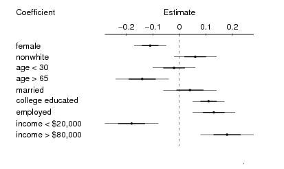
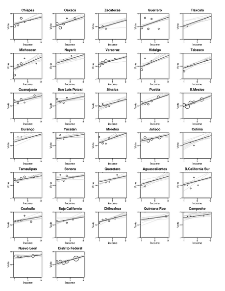
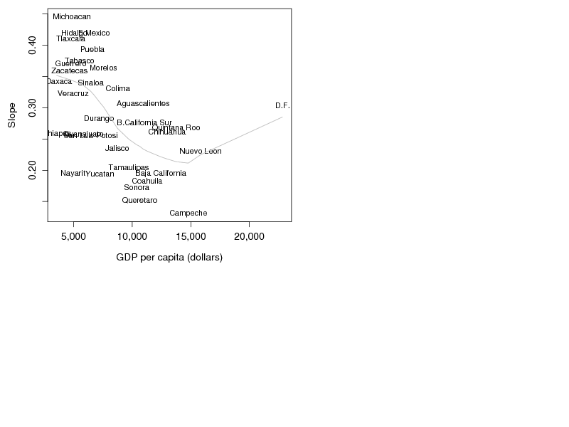
At this point I'd plot the estimates and se's vs. some group-level explanatory variable characterizing the 600 regressions. (That's the "secret weapon.") More formal steps would include running a regression of the estimated B2's on relevant group-level predictors. (Yes, if you have 600 cases, you certainly must have some group-level predictors.) And the next step, of course, is a multilevel model. But at this point I think you've probably already solved your immediate problem.

Matt Salganik is teaching introductory statistics this year and would like to do lots of class-participation activities. He came up with the idea of giving each student a mini-whiteboard (the little ones that you can affix to a refrigerator door) and marker, so that when questions come up in class, each student can sketch his or her answer and hold it up for him to see. This seems like a great idea to me. I had only two suggestions:

1. Make it one whiteboard for each pair of students. I've found that students can focus better in class when they are working in pairs--it's harder for them to just gaze off into space and give up.

2. Hand the boards out at the beginning of each lecture and have the students hand them back at the end of lecture. If you let the students keep the boards, they'll inevitably forget to bring them to class, have to borrow from each other, etc.

There's an interesting article on Wikipedia by Aaron Swartz. Swartz comes to a similar conclusion as I did--Wikipedia and traditional encyclopedias are actually structured similarly--but he approaches the question from an encyclopedia editor's point of view, whereas I was generalizing from my experience as an encyclopedia contributor. Here's what Swartz reported:

So did the Gang of 500 [central Wikipedia participants] actually write Wikipedia? Wales decided to run a simple study to find out: he counted who made the most edits to the site. . . it turns out over 50% of all the edits are done by just .7% of the users ... 524 people. ... And in fact the most active 2%, which is 1400 people, have done 73.4% of all the edits. . .

Curious and skeptical, I [Swartz] decided to investigate. I picked an article at random ("Alan Alda") to see how it was written. . . Wales seems to think that the vast majority of users are just doing the first two (vandalizing or contributing small fixes) while the core group of Wikipedians writes the actual bulk of the article. But that's not at all what I found. Almost every time I saw a substantive edit, I found the user who had contributed it was not an active user of the site. . .

If you just count edits, it appears the biggest contributors to the Alan Alda article (7 of the top 10) are registered users who (all but 2) have made thousands of edits to the site. Indeed, #4 has made over 7,000 edits while #7 has over 25,000. In other words, if you use Wales's methods, you get Wales's results: most of the content seems to be written by heavy editors. But when you count letters, the picture dramatically changes: few of the contributors (2 out of the top 10) are even registered and most (6 out of the top 10) have made less than 25 edits to the entire site. In fact, #9 has made exactly one edit -- this one! With the more reasonable metric -- indeed, the one Wales himself said he planned to use in the next revision of his study -- the result completely reverses. . . .

When you put it all together, the story become clear: an outsider makes one edit to add a chunk of information, then insiders make several edits tweaking and reformatting it. In addition, insiders rack up thousands of edits doing things like changing the name of a category across the entire site -- the kind of thing only insiders deeply care about. As a result, insiders account for the vast majority of the edits. But it's the outsiders who provide nearly all of the content. . . . Other encyclopedias work similarly, just on a much smaller scale: a large group of people write articles on topics they know well, while a small staff formats them into a single work.

I would add only one comment (besides what I wrote before). Swartz writes:

And Wikipedia should too. Even if all the formatters quit the project tomorrow, Wikipedia would still be immensely valuable. For the most part, people read Wikipedia because it has the information they need, not because it has a consistent look. It certainly wouldn't be as nice without one, but the people who (like me) care about such things would probably step up to take the place of those who had left. The formatters aid the contributors, not the other way around.

My response: I know what he's saying here, but I don't know if it's so true in general. I imagine the common format is a big part of Wikipedia's appeal--it sort of makes it into the McDonald's of information sources. I suspect that the clean and uniform format is a large part of Wikipedia's air of authority.

O'Malley and Zaslavsky recommend a scaled-inverse-Wishart model, as we discuss in Section 13.3 of our forthcoming book.. (We took the idea from an earlier draft of the O'Malley/Zaslavsky paper.) The idea is to break up the covariance matrix into a diagonal matrix of scale parameters and an unscaled covariance matrix which is given the inverse-Wishart distribution. This larger miodel is still conditionally conjugate on the larger space. The model can be thought of as a generalization of the half-t model that I describe here.

Here's the abstract for a talk in the Distinguished Lecture Series at the Computer Science department here:

I was asked by a reporter to comment on a paper by Satoshi Kanazawa, "Beautiful parents have more daughters," which is scheduled to appear in the Journal of Theoretical Biology.

As I have already discussed, Kanazawa's earlier papers ("Engineers have more sons, nurses have more daughters," "Violent men have more sons," and so on) had a serious methodological problem in that they controlled for an intermediate outcome (total number of children). But the new paper fixes this problem by looking only at first children (see the footnote on page 7).

Unfortunately, the new paper still has some problems. Physical attractiveness (as judged by the survey interviewers) is measured on a five-point scale, from "very unattractive" to "very attractive." The main result (from the bottom of page 8) is that 44% of the children of surveyed parents in category 5 ("very attractive") are boys, as compared to 52% of children born to parents from the other four attractiveness categories. With a sample size of about 3000, this difference is statistically significant (2.44 standard errors away from zero). I can't confirm this calculation because the paper doesn't give the actual counts, but I'll assume it was done correctly.

Choice of comparisons

Not to be picky on this, though, but it seems somewhat arbitrary to pick out category 5 and compare it to 1-4. Why not compare 4 and 5 ("attractive" or "very attractive") to 1-3? Even more natural (from my perspective) would be to run a regression of proportion boys on attractiveness. Using the data in Figure 1 of the paper:

Peter Woit has an interesting article--a review of a book called "The Trouble With Physics," where he talks about the struggle of a physicist named Lee Smolin to do interesting work amid the challenges of dealing with people in different subfields of physics (in particular, string theory). Smolin characterizes academic physics as "competitive, fashion-driven" and writes, "during the years I worked on string theory, I cared very much what the leaders of the community thought of my work. Just like an adolescent, I wanted to be accepted by those who were the most influential in my little circle."

I can't comment on the details of this since my physics education ended 20 years ago, but there are perhaps some similarities to statistics. But first, the key differences:

1. Statistics is a lot easier than physics. Easier to do, and easier to do research in. You really don't need much training or experience at all to work in the frontiers of statistics.
2. There's a bigger demand for statistics teachers than physics teachers. As a result, ambitious statistics Ph.D.'s who want faculty positions don't (or shouldn't) have to worry about being in a hot subfield. I mean, I wouldn't recommend working on something really boring, but just about every area in statistics is close to some interesting open problems.

Now to the issues of trends, fads, and subfields. I remember going to the Bayesian conference in Spain in 1991 and being very upset, first, that nobody was interested in checking the fits of their statistical models and, second, that there was a general belief that there was something wrong or improper about checking model fit. The entire Bayesian community (with very few exceptions, most of whom seemed to be people I knew from grad school) seemed to have swallowed whole the idea of prior distributions as "personal probability" and had the attitude that you could elicit priors but you weren't allowed to check them by comparing to data.

The field has made some progress since then--not so much through frontal attack (believe me, I've tried) as from a general diffiusion of efforts into many different applications. Every once in awhile, people applying Bayesian methods in a particular application area forget the (inappropriate) theory and check their model, sometimes by accident and sometimes on purpose. And then there are some people who we've successfully brainwashed via chapter 6 of our book. It's still a struggle, though. And don't get me started on things like Type 1 and Type 2 errors, which people are always yapping about but, in my experience, don't actually exist...

But here's the point: for all my difficulties in working with the Bayesian statisticians, things have been even harder with the non-Bayesians, in that they will often simply ignore any idea that is presented in a Bayesian framerwork. (Just to be clear: this doesn't always happen, and, again, there's a lot more openness than there used to be: as people become more aware of the arbitrariness of many "classical" statistical solutions, especially for problems with complex data structures, there is more acceptance of Bayesian procedures as a way of getting reasonable answers (as Rubin anticipated in his 1984 Annals of Statistics paper).)

Anyway, I'd rather be disagreed with than ignored, and so I realize it makes sense to do much of my communication within the Bayesian community--that's really the best option available. It's also a matter of speaking the right language; for example, when I go to econometrics talks, I can follow what's going on, but I usually have to maintain a simultaneous translation in my head, converting all the asymptotic statements to normal distributions and so forth. To communicate with those folks, I'm probably better off speaking in my own language as clearly as I can, validating my methods via interesting applications, and then hoping that some of them will reach over and take a look.

P.S. For more on why Bayes, see here and here.

Looking around, I found this by Jenny Davidson from the English department and this by Peter Woit from the math department. I know Peter and have never met Jenny Davidson, but I have to say that her blog is more readable. Literature is just more accessible than math/physics. Davidson has an entry on the swimmer Lynne Cox which was pretty cool because I remember hearing a fascinating radio interview with Cox a few years ago and wanting to learn more about her. There's really a lot of cool stuff here; I don't know how Davidson finds the time to put it all down, but I guess it's good to stay in practice if you're a professional writer. Out of curiosity, I checked her hits--she gets about the same amount of traffic as this blog, but most of the referrals are from search engines, whereas more of mine come from my own webpage or other blogs. Peter's blog is mostly about string theory, which is something I know nothing about, as my physics education ended many years ago with quantum mechanics.

This is full of cool stuff. I'll add it to the links on this blog once I figure out how to do so.

Hadar Kadar writes of a program called PDF2XL that converts pdf files of tabular data to Excel files:

Arnold Kling suggests:

Teachers should not be allowed to construct and grade their own exams. Instead, examination should be done by outsiders. . . . A simple way to separate the teacher from the exam is to exchange grading responsibilities. For example, have the teacher of "algebra 2" make up and grade the final exam given to the students taking "algebra 1" from a different teacher. Chances are, the algebra 2 teacher has a good idea of what it is really important for students to master in algebra 1. . . . With the standard practice, where professors make up their own exams, the students put pressure on the professor to make the course as easy as possible. If instead the exam were made up externally, then the pressure would be on the professor to teach the course rigorously.

This seems like a good idea. I've felt for a long time that standardized tests would improve the teaching of introductory statistics, as well as the evaluation of the teachers. Writing the standardized test is a lot of work, so I haven't done it yet, but I've been planning to do so before the next time I teach the intro course.

Here's the full text of Kling's article, all of which makes sense to me.

Steve Brooks writes,

Suppose you're fitting a simple generalized linear model with two different fixed effects each with several different levels e.g.,

Y_{ijk} ~ Poisson (L_{ij})
and log L_{ij} = a + b_i + c_j

For identifiability you need to fix a couple of parameters (e.g., b_1 = c_1 =0), but the choice of which to fix and to what value is arbitrary and will affect all of the other parameter values. This then means that the penalty from the priors differs depending on what constraints you impose and though this may not have much affect on posterior means etc. it can make a huge difference to the associated posterior model probabilities. In particular, you can calculate the model probabilities between two identical models but with different constraints (thus identical likelihood, but effectively different priors) and you get non-equal PMP's.

This is pretty basic and well-known, right, but is there a general consensus on what to do about it? If you want to compare models, there are two things you can do: (1) essentially average over all possible constraints, but then what's the theoretical justification for this; and (2) find a prior that is invariant to the constraint, but this is often tricky.

My reply:

What I would do is to model the b's and the c's (for example, b_i ~ N(mu_b, sigma^2_b), and c_j ~ N(mu_c,sigma^2_c)). The model now has redundant parameters, so then I'd identify things by defining:

a.adj <- a + mean(b[]) + mean(c[])
b.adj[i] <- b[i] - mean(b[]), for each i
c.adj[j] <- c[j] - mean(c[]), for each j

(For convenience I'm using Bugs notation.) These b.adj's and c.adj's are what I call finite-population effects. We discuss it more in our forthcoming book.

The above is the cleanest approach, I think.

Harold Doran writes,

Boris forwarded an interesting column by Arthur Brooks. I'll excerpt it, then give my thoughts. Brooks writes:

Liberal politics will prove fruitless as long as liberals refuse to multiply. . . . On the political left, raising the youth vote is one of the most common goals. This implicitly plays to the tired old axiom that a person under 30 who is not a liberal has no heart (whereas one who is still a liberal after 30 has no head). . . .

But the data on young Americans tell a different story. Simply put, liberals have a big baby problem: They're not having enough of them, they haven't for a long time, and their pool of potential new voters is suffering as a result. According to the 2004 General Social Survey, if you picked 100 unrelated politically liberal adults at random, you would find that they had, between them, 147 children. If you picked 100 conservatives, you would find 208 kids. That's a "fertility gap" of 41%. Given that about 80% of people with an identifiable party preference grow up to vote the same way as their parents, this gap translates into lots more little Republicans than little Democrats to vote in future elections. Over the past 30 years this gap has not been below 20%--explaining, to a large extent, the current ineffectiveness of liberal youth voter campaigns today.

Alarmingly for the Democrats, the gap is widening at a bit more than half a percentage point per year, meaning that today's problem is nothing compared to what the future will most likely hold. Consider future presidential elections in a swing state (like Ohio), and assume that the current patterns in fertility continue. A state that was split 50-50 between left and right in 2004 will tilt right by 2012, 54% to 46%. By 2020, it will be certifiably right-wing, 59% to 41%. A state that is currently 55-45 in favor of liberals (like California) will be 54-46 in favor of conservatives by 2020--and all for no other reason than babies.

The fertility gap doesn't budge when we correct for factors like age, income, education, sex, race--or even religion. . . .

My thoughts:

1. First off, it's interesting that these differences are so large. It would be interesting to look at these differences over time (I assume Brooks is writing a longer paper with these trends).

2 Considering this as a long-term phenomenon, I'd expect the parties to gradually move to the right to stay where the voters are. So I wouldn't think the Democrats are doomed, but rather that they'd have to move to the right as necessary. And, indeed, our calculations show that the Democrats would do better by moving slightly to the right.

3. Right now, however, the Republicans are more to the right of center than the Democrats are to the left of center (at least, as perceived by the voters on some key issues); see Figure 4 of this paper. So, in the short term, it appears that the parties are a little ahead of themselves in moving to the right.

4. I recently linked to a Pew Research Center survey that had the following result:

This would seem to contradict the idea that the youngsters are mostly Republicans. Things might change in future years, of course, but the graph suggests that things are a little more complicated than a simple inheritance of party ID.

5. Finally, political policies are also affected by factors other than public opinion. Just to consider two examples: communism and the current Iraq War are two policies that haven't seemed to work so well and have declined in popularity, presumably for policy reasons. This is mediated by public opinion but my point here is that the underlying success of various policy proposals can have an impact--it's not just party ID that will determine things. To think about this in another direction, sometimes popular positions do not get adopted (for example, raising the minimum wage in the U.S., or instituting the death penalty in Europe), partly because of interest groups, political maneuvering, external norms, etc.

Way back when, people considered the demographic trends in the other direction, and expected that universal suffrage would lead to confiscatory taxation (the lower 60% of income could tax the upper 40% out of existence, and this would just continue because the poor have more kids than the rich), but it didn't happen.

To summarize: the trends that Arthur Brooks identifies are interesting, and I'd assume they'll have some effect; at the same time, I'd be wary of using them to forecast too directly since the parties have the opportunity to change their positions while this is all happening.

This was forwarded to me. I have no connection with the project but it looks like something that could be of interest to a statistics or quantitative social science student.

Hal Stern updated our paper, 'The difference between "significant'' and "not significant'' is not itself statistically significant,' to include this example of sexual preference and birth order. Here's the abstract of our paper:

It is common to summarize statistical comparisons by declarations of statistical significance or non-significance. Here we discuss one problem with such declarations, namely that changes in statistical significance are often not themselves statistically significant. By this, we are not merely making the commonplace observation that any particular threshold is arbitrary---for example, only a small change is required to move an estimate from a 5.1% significance level to 4.9%, thus moving it into statistical significance. Rather, we are pointing out that even large changes in significance levels can correspond to small, non-significant changes in the underlying variables.

The error we describe is conceptually different from other oft-cited problems---that statistical significance is not the same as practical importance, that dichotomization into significant and non-significant results encourages the dismissal of observed differences in favor of the usually less interesting null hypothesis of no difference, and that any particular threshold for declaring significance is arbitrary. We are troubled by all of these concerns and do not intend to minimize their importance. Rather, our goal is to bring attention to what we have found is an important but much less discussed point. We illustrate with a theoretical example and two applied examples.

The full paper is here, and here are some more of my thoughts on statistical significance.

Aleks pointed me to this site by Alexander Genkin, David D. Lewis, and David Madigan that has a program for Bayesian logistic regression. It appears to allow some hierarchical modeling and can fit very large datasets. I haven't tried it out yet but it looks pretty cool. I imagine that for some complicated problems (for example, estimating state-by-state time series of public opinion), it probably wouldn't work "straight out of the box"--but that's fine, nothing else is available to solve these problems. The good news is that the program of Genkin, Lewis, and Madigan is open-source and (apparently) fast, so it could be possible and worth it to go inside and adapt its code as necessary to fit more complicated multilevel models.

P.S. Here's the paper. According to Yu-Sung, they use a one-variable-at-a-time update, so maybe some rotation would speed things up.

There's been a lot of discussion of Wikipedia compared to encyclopedias (typically, the Brittanica); see, for example, this article by Stacy Schiff in the New Yorker. The only thing I'd like to add to this discussion is that Wikipedia and traditional encyclopedias aren't that different as might be supposed. One of the features of Wikipedia is that people write the articles for free, just for the love of it. I've written several articles for encyclopedias, and it's basically the same thing. They pay a very small amount, and basically the reason for writing an article is that I tihnk somebody might read it, and I'd like to inform them. The mechanism is clearly different from Wikipedia, and the traditional encyclopedia is not infinitely updatable etc., but it's more wiki-like than one might think from the outside.

One of the most successful new internet companies, judging by the amount of traffic that they are getting, is Zillow, a real estate data company that specializes in the prices of housing. However, they have provided very interesting plots of home values in several metropolitan areas in the US. Finally, we can throw away the Boston housing dataset.

Amanda Geller writes,

I [Amanda] am using the NYC Housing and Vacancy Survey to look at the associations between disorder and crime. The city is divided into 55 neighborhoods, and in every wave, they survey about 18,000 households – about 250-300 per neighborhood. I’ve aggregated the microdata to the neighborhood level, so I have a panel of the 55 neighborhoods, over 5 waves, and my predictors are basically all rates – rates of broken windows, public assistance receipt, etc – predicting crime rates.

My problem is that the HVS, while stratified by neighborhood, is not random within neighborhood. Housing units are surveyed in clusters of 4, and unfortunately I don’t have cluster ID’s and can’t get them from the census bureau. I’ve discussed this and it sounds like because the problem boils down to measurement error in my predictors, then I don’t need to worry about bias. But what I do need to worry about are the standard errors; I need to inflate them to account for the design effect.

So the question remains on how to do this – whether I need to look at a sample of households to determine how similar the clusters are, how to measure the design effect, etc.

My reply: I think the best approach, if you can, is to gather some supplementary data to estimate the within-cluster correlations.

I noticed a link by Tyler Cowen:

A few days ago Paul Krugman argued (Times Select, or here is a Mark Thoma summary) that it matters a great deal which political party rules in the United States. Republicans tend to bring gilded ages, Democrats tend to bring greater income equality.

Cowen gives some discussion and links to other comments by Andrew Samwick, Greg Mankiw, and Matthew Yglesias, along with this overview by Brad DeLong.

Anyway, I think all these people should take a look at Larry Bartels's recent paper on income, voting, and the economy. Here's Larry's graph:

I won't repeat my summary of Larry's paper here and my further comments here except to say that, yes, sample size issues are a concern but Larry has a coherent and interesting story. Definitely worth looking at if you're interested in the topic, whatever your political perspective.

Michael Braun writes:

For the last couple of months, I've been reflecting on your recent Bayesian Analysis article on prior distributions for variance parameters in hierarchical models. As a marketing researcher who uses Bayesian methods extensively (and a recent student of Eric Bradlow), I am interested in how your findings might extend to the multivariate case. I'm hoping you can help me understand some issues related to the following problem.

Aleks pointed me toward this delightful picture:

Commenting on this entry, Matthew Shugart linked to this graph by Rici Lake on votes for the 3 parties in the recent Mexican election. Each dot on the graph represents a polling place:

This is interesting, although I don't reallly know enough to understand what is meant by comparing polling places. It would be interesting to see graphs at other levels of aggregation also.

Lots more pretty graphs here. The states shouldn't be ordered alphabetically (I'd prefer increasing order of support for PAN, for example), and I'd like the grid lines to be much lighter (in the individual-state graphs, the grid lines really obscure the dots), but that's just me being picky. The next step is to do some comparisons to 2000. Are the polling places the same? If so, it's an interesting graphical challenge because now we have 6 vote proportoins (after scaling to sum to 1 in each election, that's 4 different outcomes) for each district.

Michael Weiksner writes,

I [Weiksner] do research on deliberation, where the treatment itself is defined as the interaction with other people (who are inevitably also randomly assigned to the treatment group). Because all the treated individuals interact, I know that the safest course of action is to look only at group level effects. But that's highly unsatisfying, since you can't really shed any light on questions about individuals, like does deliberation create better citizens?

I read that, in the recent Connecticut primary election, Lamont did better in the richer towns and Lieberman did better in the poorer towns. But the exit poll showed little correlation between income and vote preference (see page 5 of this document). Putting these two facts together, I think this implies that, within towns, Lamont did better among poorer voters and Lieberman did better among richer voters.

I'd like to do more analysis (as in here and here) but I don't have the poll data and so can just speculate.

P.S. Boris pointed out Mark Blumenthal's comments here and here on exit polls and voting in Connecticut.

Dan Goldstein links to this new online journal on decision analysis. It looks pretty interesting. I am positively disposed toward this article by Davd Gal, since what is often described as "loss aversion" is often better characterized as "uncertainty aversion" (see here, for example).

A couple people pointed me to this, which relates to this (scroll down to the section on Sociological Methodology).

I just have a couple of comments:

1. Given that this is a sociological journal, I don't think Heckman should have been surprised that they got a sociologist to discuss his paper. I'm not clear what he means by "world-class credentials." I think it was generous of Heckman to write the article for Sociological Methodology, and I assume that a primary reason for writing the article was to convey his point of view to the quantitative sociologists. With this in mind, it makes sense that a sociologist be the discussant.

2. The email exchanges are pretty hard to follow. I think this is often the case with email exchanges: everything seems so clear at the time, but later--or to others--it's difficult to understand what was going on at the time.

For my part, I am glad that Heckman's article, Sobel's discussion, and Heckman's rejoinder finally did get published, since they raise some interesting issues about modeling and causal inference. As I noted earlier, Heckman's anti-experimentation position is something we rarely see in statistics, so it is good to see it argued (and counter-argued) so forecefully. Michael Sobel is a colleague of mine at Columbia, and I think I did see an earlier draft of his discussion at some point. I would think that it's good for Heckman, as well as the statistical community, to have these ideas out there, so it all seems to have worked out ok (although with too much trauma to all participants, it appears).

I'll plug this book (coauthored with Jennifer Hill) more fully when it's closer to print (it's scheduled to physically appear in book form in October). I'm posting this now to let anyone know that if you're interested in using it as a textbook for the fall, you can contact me and I can arrange with the publisher to make sure that your students get photocopies in time for the beginning of the semester.

Here's the table of contents.

Tian asks a question about multilevel modeling:

Suppose you have 50 state-level effects parameters. If you treat them as fixed effects and assume non-informative priors, this should just be equivalent to compute the regular likelihood function, right?

If these 50 parameters are regarded as random effects and there is a hyper-distribution for them, say a normal, then the bell-shape of the normal distribution will lead to milder differences between these parameters. Would this fall under the argument of having parsimonious models?

This reminds me of a few things. First, I remember when I was in an oral exam at Berkeley. The student, not of one of my own advisees, was fitting a multilevel regression with varying intercepts for the 50 states, and one of the examiners said that he wasn't sure he believed the exchangeability assumption. I pointed out that "exchangeability" refers to invariance to permutations of indexes, and thus alternative classical analyses (no pooling, complete pooling) also are exchangeable--they are just special cases of the multilevel model where the group-level variance is infinity or zero. (Yes, I know that by giving the story from my perspective, I'm being self-serving, but what choice do I have here?)

Nonparametric?

Getting back to Tian's question, this is something I've thought about for awhile, that hierarchical models are, in fact, nonparametric. I don't actually think the term "nonparametric" is clearly defined. Sometimes it refers to statistical procedures in which no parameters are estimated, other times it refers to settings where the number of parameters is infinite, or potentially infinite. One way to characterize nonparametric models is that the resulting inferences are not limited to any parametric form. In that sense, hierarchical (multilevel) Bayesian estimates are indeed nonparametric. The model that they are pooling toward is parametric, but the actual estimates are nonparametric in the sense that all things are possible, depending on how much pooling is done.

This was made clear to me in the research that led to my 1990 Jasa paper (with Gary King): By setting up a hierarchical model, we were not limiting the seats-votes curve to any particular parametric form. That made our model more appealing (at least from my perspective) than its predecessors in the seats-votes literature, where various parametric forms were assumed. I think it's cool that parametric modeling can be used in the service of nonparametric inferences.

This blog entry by Tyler Cowen reminded me of the course that Seth Roberts and I once taught on left-handedness. The main things I remember learning:

1. Left-handedness is not the opposite of right-handedness. Most righties do everything with their right hand, but lefties are mostly mixed. Also, left-handers are typically OK with their right hands, but righties are typically not so good the other way. Related to this is that there's really not such a thing as "ambidextrous": the term "mixed-handed" is better: people who use different hands for different tasks are usually OK with either hand.

2. This is more of a "folk psychology" thing, but it's interesting: a lot of people, especially lefties, either want to know the "rule" for determining whether someone is left-handed, or think there is such a rule. Many people aren't comfortable with the idea of a continuum, and want this to be a binary variable. (Interestingly, I even ran across a statistics textbook once that (mistakenly) characterized handedness as an example of a categorical variable.)

3. The studies that find lefties to die younger are interesting. Not airtight, but not trivially demolishable, either. At least as of my reading in 1994, the case is still open on this one.

4. We did a little study in our class (approx 20 students, about 1/4 righties and the rest left- or mixed-handed), asking each student to make a list of his or her closest friends (outside of the class itself) and then give them the handedness inventory (a standard 10-question battery that yields a handedness score between -1 and 1). We found a statistically significant correlation between the handedness of the people in the class and the average handedness scores of their friends. We never followed this up with further studies, though.

5. In reading the papers for the class, I noticed that many were written by scientists from Canada and New Zealand, not much from the U.S. I asked Seth why, and he said it's because you can study handedness with a low budget.

6. We were featured in the local papers as an example of a fun college class. But there was one media outlet that contacted us, I don't remember which one, which Seth suspected was trying to use us as an example of the crap that gets taught in college nowadays. I was careful to be very boring when talking with this reporter so that he wouldn't get any incriminating quotes from me. Also, a local TV station wanted to come and shoot one of our classes, but they decided not to when I explained that we weren't really focusing on original research--the course was mostly discussions of existing articles. (It was a good class, though, I think.)

There's an article by Abhijit Vinayak Banerjee in the Boston Review recommending randomized experiments (or the next best thing, "natural experiments") to evaluate stragies for foreign aid. Also, here's a link to the Boston Review page which includes several discussions by others and a response by Banerjee.

On the specific topic of evaluating social interventions, I have little to add beyond my coments last year on Esther Duflo's talk: randomized experimentation is great, but once you have the randomized (or "naturally randomized") data, it still can be a good idea to improve your efficiency by gathering background inforomation and using sophisticated statistical methods to adust for imbalance. To quote myself on Dfulo's talk:

There are a couple ways in which I think the analysis could be improved. First, I'd like to control for pre-treatment measurements at the village level. Various village-level information is available from the 1991 Indian Census, including for example some measures of water quality. I suspect that controlling for this information would reduce the standard errors of regression coefficients (which is an issue given that most of the estimates are less than 2 standard errors away from 0). Second, I'd consider a multilevel analysis to make use of information available at the village, GP, and state levels. Duflo et al. corrected the standard errors for clustering but I'd hope that a full multilevel analysis could make use of more information and thus, again, reduce uncertatinties in the regression coefficients.

Why don't we practice what we preach?

Nonetheless, I am not sure myself that large-N studies are always a good idea. And, in practice, I rarely do any sort of formal experimentation when evaluating interventions in my own activities. Here I'm particularly thinking of teaching methods, where we try all sorts of different things but have difficulty evaluating what works. I certainly do make use of the findings of educational researchers (many of whom, I'm sure, use randomized experiments), but when I try things out myself, I don't ever seem to have the discipline to take good measurements, let alone set up randomized trials. So in my own professional life, I'm just as bad as the aid workers who Banerjee criticizes for not filliong out forms.

This is not meant as a criticizm of Banerjee's paper, just a note that it seems easier to give statistical advice to others than to follow it ourselves.

Albyn Jones sent me this link by Hans Rosling, the founder of Gapminder. It's a great demonstration of statistical visualization. I'd like to use it to start off my introductory statistics classes--except then the students would probably be disappointed that my lectures aren't as good...

Some good news:

The Bill and Melinda Gates Foundation, run by the chairman of the Microsoft Corporation, will deliver $287 million in five-year grants to researchers working to produce an AIDS vaccine. The caveat: Grantees must agree to pool their results. Fragmented and overlapping work in the area of AIDS research has hindered progress toward a vaccination for the virus that affects 40 million people around the world.... A web site will share data in real time.

More at The Wall Street Journal and at YaleGlobalOnline.

Hopefully this will push the work towards my vision of the interactive analysis of data through the internet instead of the current model of only publishing the not-always-reproducible results of the analysis. See my previous postings on statistical data.

Jason Anastasopoulos writes,

I [Jason] have just finished uploading an online internet questionnaire that is to be used for social science research in the near future. Could you possibly post a link to the survey on your blog and ask users to take the survey and offer any comments, suggestions etc?

Here it is.

Richard Zur writes,

Are any Bayesian estimates invariant to parameterization? If not, what do people do about it?

I was planning on constructing an informative prior in one parameterization and then reparameterizing into something more convenient. I was planning on using a MAP estimate to compare to the MLE, but now I'm worried because MAP is not invariant. What about mean, median, variance, etc? Do people deal with this issue anywhere? Would delving into the invariant prior literature help? Mostly they seem to focus on non-informative priors, as far as I can see.

My quick answer is that it's ok for things to depend on parameterization; that is in fact a key way in which information is encoded in a model. Even linear transformations can affect how parameters are interpreted and how models are selected, thus affecting the final inferences. I'm not a big fan of invariant prior distributions (although we do discuss the topic briefly in Chapter 2 of Bayesian Data Analysis).

I'll also use this to promote one of my favorite papers, Parameterization and Bayesian Modeling. Here's the abstract:

Progress in statistical computation often leads to advances in statistical modeling. For example, it is surprisingly common that an existing model is reparameterized, solely for computational purposes, but then this new conŽ guration motivates a new family of models that is useful in applied statistics. One reason why this phenomenon may not have been noticed in statistics is that reparameterizations do not change the likelihood. In a Bayesian framework, however, a transformation of parameters typically suggests a new family of prior distributions. We discuss examples in censored and truncated data, mixture modeling, multivariate imputation, stochastic processes, and multilevel models.

and here's the paper.

Matt Salganik has posted the estimates of the number of acquaintances (the so-called "degree distribution") for a random sample of Americans. These estimates come from the analysis of Tian Zheng, Matt, and myself of survey data by Killworth, McCarty et al. that just appeared in the Journal of the American Statistical Association.

Here are the estimated distributions:

but the data are actually better than this because they have estimates along with background information on 1370 respondents, so you can do analyses like this regression of log (#acquantainces):

Three guys were walking together, and one said to another,

Lemme tell ya something. If there was a Jesus for wiseasses, it'd be you.

I don't know what that means, but it sounded good.

Nuno Teixeira writes,

After knowing about Google Trends (as far as I can remenber, from your blog), I've spent some of my time around it. One interesting trend emerges when you search for "sex" and "love". For instance, you can check that the search volume for "sex" increases around the middle of each year (at least, the years covered by Google trends), this is, around spring and summer. Curiously enough, a month or two later, you can find an increase in the search volume for "love". By the way, similar results emerge with the same words on Portuguese.

Of course, there is no objective basis to take these trends to much serious, and probably they are just a funny little bit of data. However, I would like to hear from you, someone used to deal proficiently with statistical data, some opinions.

I have no ideas on this at all. But I was motivated to play around with Google Trends. "Statistics" also has strong seasonal patterns, with a broad dip in the spring-summer and a steep drop around Christmas. "Bayes" just shows a steady decline. "Causal" drops at Christmas too, as does "social science." OK, I better stop now.

Mathis Schulte writes,

Here's the paper, (by Jeff Cai and myself) and here's the abstract:

Could John Kerry have gained votes in the recent Presidential election by more clearly distinguishing himself from George Bush on economic policy? At first thought, the logic of political preferences would suggest not: the Republicans are to the right of most Americans on economic policy, and so in a one-dimensional space with party positions measured with no error, the optimal strategy for the Democrats would be to stand infinitesimally to the left of the Republicans. The median voter theorem suggests that each party should keep its policy positions just barely distinguishable from the opposition.

In a multidimensional setting, however, or when voters vary in their perceptions of the parties' positions, a party can benefit from putting some daylight between itself and the other party on an issue where it has a public-opinion advantage (such as economic policy for the Democrats). We set up a plausible theoretical model in which the Democrats could achieve a net gain in votes by moving to the left on economic policy, given the parties' positions on a range of issue dimensions. We then evaluate this model based on survey data on voters' perceptions of their own positions and those of the candidates in 2004.

Under our model, it turns out to be optimal for the Democrats to move slightly to the right but staying clearly to the left of the Republicans' current position on economic issues.

I'll be speaking on August 13 at the American Sociological Association meeting in Montreal. I'll start with our red-state, blue-state analysis and then talk about some more recent work along these lines, including our anlaysis of Mexican voting data. Since it's a methodological session, I'll be focusing on some of the challenges we've faced in understanding and checking the varying-intercept, varying-slope multillevel models that we've been using. Any sociologists who are reading this: you have a couple of weeks to prepare some good questions...

Matthew Hurst points to a gallery of business-style visualizations at Perceptual Edge. There are a few conclusions that can be made from Stephen Few's examples. In particular, Stephen does a good job designing graphs and tables that enable the analyst to quickly obtain answers to interesting questions:

• Rank numerical values as to speed up answering questions such as "Who's the best? Who's the worst? Who's second best? What's the difference between the first and the second?" #1,#8
• 3D charts may be flashy, but our perception is 2D. If the table has several dimensions, stratify by the order of importance. In #3, the location is deemed more important than the year.
• If there are too many comparisons to be made within a single graph, focus on pairwise comparisons and prepare a series of graphs. #6,#7
• While example #4 may seem to claim that tables are superior to graphs, Stephen's own example invalidates this claim very well.
• Do not clutter the display: instead prepare several different views of the same data #2
• Horizontal bargraphs often work better than pie charts. #5

Another important heuristic in the design of graphs is to include helpful elements that cross-index the quantities (color denoting type) #2. At the same time, one shouldn't overload the analyst's perception with irrelevant distinctions, such as using color to indicate an irrelevant quantity (#4).

Lenore Fahrig writes,

I have two multinomial logistic models meant to explain the same data set. The two models have different predictor variables but they have the same number of predictor variables (2 each). Can I use the difference in deviance between the two models to compare them?

This sort of question comes up a lot. My quick answer is to include all four predictors in the model, or to combine them in some way (for example, sometimes it makes sense to reparameterize a pair of related predictors by considering their average and their difference). I can see why it can be useful to look at the improvement in fit from adding a predictor or two, but I don't see the use in comparing models with different predictors. (I mean, I see how one can learn interesting things from this sort of comparison, but I don't see the point in a formal statistical test of it, since I would think of your two original models as just the starting points to something larger.)

Jeremy Miles forwards this article from the New Scientist:

The legend of Manfred von Richthofen, aka the Red Baron, has taken a knock. The victories notched up by him and other great flying aces of the first world war could have been down to luck rather than skill.

Von Richthofen chalked up 80 consecutive victories in aerial combat. His success seems to suggest exceptional skill, as such a tally is unlikely to be down to pure luck.

However, Mikhail Simkin and Vwani Roychowdhury of the University of California at Los Angeles think otherwise. They studied the records of all German fighter pilots of the first world war and found a total of 6745 victories, but only about 1000 "defeats", which included fights in which pilots were killed or wounded.

The imbalance reflects, in part, that pilots often scored easy victories against poorly armed or less manoeuvrable aircraft, making the average German fighter pilot's rate of success as high as 80 per cent. Statistically speaking, at least one pilot could then have won 80 aerial fights in a row by pure chance.

The analysis also suggests that while von Richthofen and other aces were in the upper 30 per cent of pilots by skill, they were probably no more special than that. "It seems that the top aces achieved their victory scores mostly by luck," says Roychowdhury.

I'm still confused. (6745/7745)^80 = .000016, or 1 in 60,000. Still seems pretty good to me. I mean, with these odds I wouldn't put my money on Snoopy, that's for sure.

I just reviewed a paper for a statistics journal. My review included the following sentences which maybe I should just put in my .signature file:

The main weakness of the paper is that it does not have any examples. This makes it hard to follow. As an applied statistician, I would like an example for two reasons: (a) I would like to know how to apply the method, and (b) it is much easier for me to evaluate the method if I can see it in an example. I would prefer an example that has relevance for the author of the paper (rather than a reanalysis of a "classic" dataset), but that is just my taste.

Lest you think I'm a grouch, let me add that I liked the paper and recommended acceptance. (Also, I know that I do not always follow my own rules, having analyzed the 8 schools example to death and having even on occasion reanalyzed data from Snedecor and Cochran's classic book.)

Peter Yared pointed me to these maps that he made showing various characteristics of U.S. states (from Census data) that have similar patterns to the votes for Democrats and Republicans in recent Presidential elections (that is, comparisons of the coasts and industrial midwest to the southern and central states). Many of these relate to the well-known recent correlation between state income and support for the Democrats. The patterns at the individual levels may differ, though. At a policy level, it makes sense that the Republicans favor transfer payments to poor states but not to poor people; with the reverse pattern for the Democrats.

This article by Donald Kinder is an interesting review of research on political views as they are inherited and as they develop with age. I also like it because he refers to my sister's work on the essentialist beliefs of children.

I'll have to think a bit about how this all relates to this picture of party ID and age:

(see also the other data here).

I received the following (unsolicited) email:

Eduardo linked to this interesting paper by Walter Mebane on using Benford's Law (the distribution of digits that arises from numbers that are sampled uniformly on a logarithmic scale) to investigate election fraud. I'll give my thoughts, but first here's the abstract:

This paper, "Biological versus nonbiological older brothers and men's sexual orientation," by Anthony Bogaert, appeared recently in the Proceedings of the National Academy of Sciences and was picked up by several news organizations, including Scientific American, New Scientist, Science News, and the CBC. As the Science News article put it,

The number of biological older brothers correlated with the likelihood of a man being homosexual, regardless of the amount of time spent with those siblings during childhood, Bogaert says. No other sibling characteristic, such as number of older sisters, displayed a link to male sexual orientation.

I was curious about this--why older brothers and not older sisters? The article referred back to this earlier paper by Blanchard and Bogaert from 1996, which had this graph:

and this table:

Here's the key quote from the paper:

Significant beta coefficients differ statistically from zero and, when positive, indicate a greater probability of homosexuality. Only the number of biological older brothers reared with the participant, and not any other sibling characteristic including the number of nonbiological brothers reared with the participant, was significantly related to sexual orientation.

The entire conclusions seem to be based on a comparison of significance with nonsignificance, even though the differences do not appear to be significant. (One can't quite be sure--it's a regression analysis and the different coef estimates are not independent, but based on the picture I strongly doubt the differences are significant.) In particular, the difference between the coefficients for brothers and sisters does not appear to be significant.

What can we say about this example?

As I have discussed elsewhere, the difference between "significant" and "not significant" is not itself statistically significant. But should I be such a hard-liner here? As Andrew Oswald pointed out, innovative research can have mistakes, but that doesn't mean it should be discarded. And given my Bayesian inclinations, I should be the last person to discard a finding (in this case, the difference between the average number of older brothers and the average number of older sisters) just because it's not statistically significant.

But . . . but . . . yes, the data are consistent with the hypothesis that only the number of older brothers matters. But the data are also consistent with the hypothesis that only the birth order (i.e., the total number of older siblings) matters. (At least, so I suspect from the graph and the table.) Given that the 95% confidence level is standard (and I'm pretty sure the paper wouldn't have been published without it), I think the rule should be applied consistently.

To put it another way, the news articles (and also bloggers; see here, here, and here) just take this finding at face value.

Let me try this one more time: Bogaert's conclusions might very well be correct. He did not make a big mistake (as was done, for example, in the article discussed here). But I think he should be a little less sure of his conclusions, since his data appear to be consistent with the simpler hypothesis that it's birth order, not #brothers, that's correlated with being gay. (The paper did refer to other studies replicating the findings, but when I tracked down the references I didn't actually see any more data on the brothers vs. sisters issue.)

Warning: I don't know what I'm talking about here!

This is a tricky issue because I know next to nothing about biology, so I'm speaking purely as a statistician here. Again, I'm not trying to slam Bogaert's study, I'm just critical of the unquestioning acceptance of the results, which I think derives from an error about comparing statistical significance.

David Kane writes,

I [Kane] am putting together a class on Rhetoric which will look the ways we use words, numbers and pictures to persuade. The class will have mininal prerequisites (maybe AP Stats or the equivalent) and will be discussion/tutorial based. For the sections on numbers and pictures, I plan on assigning "How To Lie with Statistics" by Huff and "The Visual Display of Quantitative Information" by Tufte. (The students will also be learning R so that they can produce some pretty pictures of their own. The course objectives are ambitious.)

Question: What other readings might people suggest? I am especially interested in readings that are either "classic" or freely available on the web.

I hope to teach the students are to attack and defend things like the IPCC report on global warming, the EPA report on secondhand smoke and so on.

Any suggestions would be much appreciated.

My response: I can't actually think of any great examples, partly because once an issue seems clear, one way or another, persuasive reasoning seems almost a separate issue from quantitative reasoning. (I suppose this is parallel to the idea in science that if you do an experiment well, you don't need statistics because the result will jump out at you.)

OK, I'll give one recommendation: chapter 10 of my book on teaching statistics. Here are the table of contents and index for the book. I really like the index--I think it's actually fun to read.

You ask for resources on the web. I suppose it won't hurt to post one chapter . . . so here's the aforementioned Chapter 10. (The images are clearer in the published book, but I think the pdf gives the general impression.) I hope you find it useful.

Frederick Mosteller passed away yesterday. He was a leader in applied statistics and statistical education and was a professor of statistics at Harvard for several decades. Here is a brief biography by Steve Fienberg, and here are my own memories of being Fred's T.A. in the last semester that he taught statistics. I did not know Fred well, but I consider him an inspiration in my work in applied statistics and statistical education.

A Bayesian prior characterizes our beliefs about different hypotheses (parameter values) before seeing the data. While some (subjectivists) attempt to elicit informative priors systematically - anticipating certain hypotheses and excluding others - others (objectivists) prefer noninformative priors with desirable properties, letting the data "decide". Yet, one can actually use the data to come up with an informative prior in an objective way.

Let us assume the problem of modeling the distribution of natural numbers. We do not know the range of natural numbers a priori. What would be a good prior? A uniform prior would be both improper (non-normalized), but also inappropriate: not all natural numbers are equally prevalent. A reasonable prior would be an aggregate of natural number distributions across a large number of datasets.

Dorogovtsev, Mendes and Oliveira have used Google for assessing the Frequency of occurrence of numbers in the World Wide Web. While they were not concerned about priors, their resulting distribution is actually a good general prior for natural numbers. Of course, it would help knowing if the natural numbers are years or something else, but other than that, the general (power law) distribution of p(n) ~ 1/sqrt(n) is both supported by data and mathematically elegant:

In this context it is worth mentioning also Benford's law, which elaborates on an observation that the leading digits are not equally likely. Instead, 1 is considerably more likely than 9.

I came across this picture posted by Steve Hulett on the Animation Guild blog:

(See here for a bigger image.) Uncle Woody (he was born in 1916 and was named after Woodrow Wilson. It could've been worse--his sister Lucy was named after Luther Burbank, and her full name is Lutheria) worked in animation--we were always told that he drew the "in-between" drawings for cartoons--and worked on promotions for Topps gum for many years:

Wacky Packs were the biggest thing when I was in elementary school but I never knew that Uncle Woody had worked on them.

Using multilevel modeling of state-level economic data and individual-level exit poll data from the 2000 Mexican presidential election, we find that income has a stronger effect in predicting the vote for the conservative party in poorer states than in richer states---a pattern that has also been found in recent U.S. elections. In addition (and unlike in the U.S.), richer states on average tend to support the conservative party at higher rates than poorer states. Our findings are consistent with the 2006 Mexican election, which showed a profound divide between rich and poor states. Income is an important predictor of the vote both at the individual and the state levels.

Here's the paper, and here's the key graph:

The little circles in the plots show the data from the exit poll from the 2000 election (average vote plotted vs. income category within each state, with size of the circles proportional to the number of survey respondents it represents). Party is coded as 1=PRD, 2=PRI, 3=PAN, so higher numbers are more conservative. The solid line in each plot represents the estimated relation between vote choice and income within the state (as fitted from a multilevel model). The gray lines represent uncertainty in the fitted regression lines.

The graph shows the 32 states (including Mexico, D.F.) in increasing order of per-capita GDP. The slopes are higher--that is, income is a stronger predictor of the vote--in poor states. Income is a less important predictor in the rich states (except for the capital, Mexico, D.F., which has its own pattern).

Here's a plot of the slopes vs. per-capita GDP in the 32 states:

The conservative party did better with rich voters everwhere, but individual income is a much stronger predictor of the vote in poor states than in rich states. This is similar to the pattern we found in the U.S. One difference between the two countries is that in the U.S., the conservative party does better in the poor states, but in Mexico, the conservative party does better in the rich states. But at the level of individual voting, the patterns in the two countries seems similar.

We plan to replicate our study with 2006 exit polls, once we can get our hands on the data.

I was just fitting a model and realizing that some of the graphs in my paper were all wrong--we seem to have garbled some of the coding of a variable in R. (It can happen, especially in multilevel models when group indexes get out of order.) But the basic conclusion didn't actually change. This flashed me back to when Gary and I were working on our seats-votes stuff (almost 20 years ago!), and we joked that our results were invariant to bugs in the code.

Sheena Iyengar is a professor of psychology in the business school here who has worked on some interesting projects (including the speed-dating experiment). She writes,

I [Sheena] am looking for an ambitious, dedicated, and promising graduating senior interested in a full-time research assistant position for one to two years beginning August 1, 2006. Potential applicants should have a degree in either social/cognitive psychology or economics with an interest in the intersection of economics and the psychology of judgment and decision making. Preference is given to candidates with a strong math background and good writing skills who have had some research experience in a laboratory already.

The salary for this position is $45,000 and includes all health benefits. The research assistant will be responsible for running experiments, managing a laboratory, conducting statistical analyses, and will have the opportunity to co-author in journal publications. It is a truly excellent opportunity for someone who is interested in pursuing a Ph.D. in behavioral economics, psychology, and/or related disciplines. If you are interested in applying for this position, please e-mail me, Professor Sheena S. Iyengar, at ss957@columbia.edu or call at 212 854-8308. I will be interviewing potential applicants immediately.

It looks interesting to me . . .

In googling for "parking lot Stolzenberg," I came across a series of articles in the American Sociological Review on the measurement of church attendance in the United States--an interesting topic in its own right and also a great example for teaching the concept of total survey error in a sampling class. The exchange begins with an article by C. Kirk Haraway, Penny Long Marler, and Mark Chaves in 1993:

Characterizations of religious life in the United States typically reference poll data on church attendance. Consistently high levels of participation reported in these data sug-gest an exceptionally religious population, little affected by secularizing trends. This picture of vitality, however, contradicts other empirical evidence indicating declining strength among many religious institutions. Using a variety of data sources and data collection procedures, we estimate that church attendance rates for Protestants and Catholics are, in fact, approximately one-half the generally accepted levels.

Jorge Lopez sent me the following report analyzing results from the recent Mexican election. He looked at the vote totals as they emerged through the election night, and saw patterns that led him to conclude that there was fraud in the vote counting. His report begins:

Many of us took advantage of the latest technology and followed last Sunday’s elections in Mexico through a novel method: web postings of the votes through the Program of Preliminary Results, or PREP by its Spanish initials. What Mexico’s Federal Electoral Institute (IFE) did not take into account is that the postings were not only informing, they were providing valuable data that can be –and was- examined to check its “health”. The bottom line is that the data presented is ill, so ill that it appears to have been given artificial life by a computer algorithm.

What the web surfers saw is that after an initial strong showing, which began at Sunday noon with a Calderon advantage of more than 4% over López Obrador (“AMLO”), the lead began to decrease in percentages. The diminishing trend continued and, around midnight, many of us went to bed forecasting a tie by 3:00 AM Monday, and an AMLO advantage of about 1% by wake up time on Monday. The morning surprise was that the trend had changed overnight and Calderon appeared with a slim but invariant advantage of about 1%; this sent many of us to what we, physics professors, do for a living: data analysis.

. . .

Here's the full report.

I looked at the report, and I don't think it represents convincing evidence of data manipulation. There are three reasons why I say this:

1. The report doesn't have information on where the election returns came from. Thus, the changes in the votes (going one way, then reversing, etc, as shown on page 4) could arise from votes coming from different places.

2. It's not such a surprise that the vote total will become more stable over time, because the vote total at time t+1 mostly comes from the vote total at time t. So I don't see the correlation of .9999 as necessarily being meaningful.

3. In the picture on page 3, there's no particular reason to expect a normal distribution. You will see differences of close to zero in percent as the counts go on over time.

The data being analyzed remind me of an analysis I did a few years ago of a local election in New York City; see this paper ,which appeared in Chance (and also will appear in Chapter 2 in our forthcoming book).

As I told Jorge, although I disagree with his conclusions, it's good to air these things and let people make their own judgments, hence this blog posting. Jorge also send me this document from Eduardo Trejo which has some of the preliminary vote counts. Jorge also asked that if anyone has any comments, they can post them on this blog and also can send him email.

(For some more background on allegations of fraud in the Mexican election, see this Boingboing entry by Xeni Jardin, which has link to more stuff.)

I'm sometimes asked if I can recommend a statistical consultant. Rahul Dodhia is a former student (and coauthor of this paper on statistical communication) who, after getting his Ph.D. in psychology, has worked at different places including NASA, Ebay, and Amazon. He does statistical consulting; see here. I also have some colleagues in the Columbia faculty who do consulting. Rahul's the one with the website, though.

I have always been taught that the randomized experiment is the gold standard for causal inference, and I always thought this was a universal view. Not among all econometricians, apparently. In a recent paper in Sociological Methodology, James Heckman refers to "the myth that causality can only be determined by randomization,
and that glorifies randomization as the ‘‘gold standard’’ of causal inference."

It's an interesting article because he takes the opposite position from all the statisticians I've ever spoken with (Bayesian or non-Bayesian). Heckman is not particularly interested in randomized experiments and does not see them as any sort of baseline, but he very much likes structural models, which statisticians are typically wary of because of their strong and (from a statistical perspective) nearly untestable assumptions. I'm sure that some of this dispute reflects different questions that are being asked in different fields.

Heckman's article is a response to this article [link fixed--thanks Alex] by Michael Sobel, who argues that Heckman's methods are actually not so different from the methods commonly used in statistics. It's all a bit baffling to me because I actually thought that economists were big fans of randomized experiments nowadays.

P.S. As noted by an anonymous commenter, some controversy arose from this issue of Sociological Methodology, but I'm not going into detail here since said controversy is not very relevant to the scientific issues that arise in these papers, which is what I wanted to post on.

Christian Robert sent this along:

Post-doctoral position in statistical cosmology

ECOSSTAT Program National Research Agency - CNRS: Measuring cosmological parameters from large heterogeneous surveys

The ECOSSTAT program is an inter-disciplinary three year project between astrophysicists and statisticians that aims at refining the constraints on the values of parameters in the cosmological model.

Cajo Ter Braak just published this paper in Statistics and Computing. It's an automatic Metropolis-like algorithm that seems to automatically work to perform adaptive jumps. Perhaps could be useful in a Umacs or Bugs-like setting? Here's the abstract:

OK, this one is for hard-core Bayesians only . . . it's some info from Brad Carlin, Nicky Best, and Angelika van der Linde on the deviance information criterion (DIC):

Graham Webster pointed me to this interesting site that's full of data and graphs. Should be great for teaching, and for research too, in enabling people to look up and graph data quickly.

I'd like to develop some homework assignments and class-participation activities based on this site. We should be able to do better than to tell students: Hey, look at this, it's cool!

To start with, one could set students on to it and ask them to find pairs of variables with negative correlations, or pairs of variables that are approximately independent, or pairs that have zero correlation but are not independent. Or one student could pick a pair of variables, and the other could guess the regression slope.

I'm sure more could be done: the challenge is to get the students to be thinking hard, and anticipating the patterns before they see the data, rather than simply passively looking at cool patterns.

Andrew Oswald (author of the paper that found that parents of daughters are further to the left, politically, than parents of sons) writes,

I read your post on Kanazawa. I don't know whether his paper is correct, but I wanted to say something slightly different. Here is my concern.

The whole spirit of your blog would have led, in my view, to a rejection of the early papers arguing that smoking causes cancer (because, your eloquent blog might have written around 1953 or whenever it was exactly, smoking is endogenous). That worries me. It would have led to many extra people dying.

I can tell that you are a highly experienced researcher and intellectually brilliant chap but the slightly negative tone of your blog has a danger -- if I may have the temerity to say so. Your younger readers are constantly getting the subtle message: A POTENTIAL METHODOLOGICAL FLAW IN A PAPER MEANS ITS CONCLUSIONS ARE WRONG. Such a sentence is, as I am sure you would say, quite wrong. And one could then talk about type one and two errors, and I am sure you do in class.

Your blog is great. But I often think this.

I appreciate it is a fine distinction.

In economics, rightly or wrongly, referees are obsessed with thinking of some potential flaw in a paper. I teach my students that those obsessive referees would have, years ago, condemned many hundreds of thousands of smokers to death.

I replied as follows:

Jorge Bravo pointed me to this report by some statisticians (Miguel Cervera Flores, Guillermina Eslava Gomez, Ruben Hernandez Cid, Ignacio Mendez Ramirez, and Manuel Mendoza Ramirez) on the very close Mexican election. (Here's the report at its original url.)

Here are their estimated percentages for each party:

and here's the graphical version, just comparing PAN to PRD:

I can't actually figure out exactly where these estimates come from, or what exactly they are doing to get the robust, classical, and Bayesian estimates. But they should give their estimates for the difference between the two leading parties, I think, rather than separate intervals for each.

I just heard, on the radio, the recent Mexican election, which was almost tied, described as a "worst case scenario." It's a funny thing, though: a very close election is a bad thing in that it can lead to controversy, lack of legitimacy of the government, and sensitivity of results to cheating. On the other hand, a key premise of democracy is that your vote can matter, which means there has to a be a chance that the election is really close. So, the ideal seems to be an election that, before the election, is highly likely to be close, but after the election, never ends up actually being close. This is hard to arrange, though!

It's a paradox, along the lines of: you should live each day as if it were your last, but you don't want it to actually be your last...

Don't let this distract you from the more serious items on this blog.

The blog is fully working, so your comments will be processed again. And have a fun 4th-of-July weekend!

As discussed here, I've been interested in finding studies of the costs and benefits of approvals of new medical treatments, but not in the narrow sense of the costs and benefits to those being treated, but the larger balance sheet, incluing costs of running the study, risks to participants, and likely gains to the general population. (For example, approving a study early allows for potentially more gains to the general population but also more risks of unforseen adverse events.)

Jim Hammitt pointed me to this paper by Tomas J. Philipson, Ernst R. Berndt, Adrian H. B. Gottschalk, Matthew W. Strobeck, entitled "Assessing the Safety and Efficacy of the FDA: The Case of the Prescription Drug User Fee Acts." Here's the summary of the paper, and here's the abstract:

The US Food and drug Administration (FDA) is estimated to regulate markets accounting for about 20% of consumer spending in the US. This paper proposes a general methodology to evaluate FDA policies, in general, and the central speed-safety tradeoff it faces, in particular. We apply this methodology to estimate the welfare effects of a major piece of legislation affecting this tradeoff, the Prescription Drug User Fee Acts (PDUFA). We find that PDUFA raised the private surplus of producers, and thus innovative returns, by about $11 to $13 billion. Dependent on the market power assumed of producers while having patent protection, we find that PDUFA raised consumer welfare between $5 to$19 billion; thus the combined social surplus was raised between $18 to $31 billions. Converting these economic gains into equivalent health benefits, we find that the more rapid access of drugs on the market enabled by PDUFA saved the equivalent of 180 to 310 thousand life-years. Additionally, we estimate an upper bound on the adverse effects of PDUFA based on drugs submitted during PDUFA I/II and subsequently withdrawn for safety reasons, and find that an extreme upper bound of about 56 thousand life-years were lost. We discuss how our general methodology could be used to perform a quantitative and evidence-based evaluation of the desirability of other FDA policies in the future, particularly those affecting the speed-safety tradeoff.

I haven't read the paper (that takes more effort than linking to it!) but I like that they're trying to measure all the costs and benefits quantitatively.

I got the following (unsolicited) email from a publisher today:

We are developing a new, introductory statistics textbook with a data analysis approach, and would value your answers to our brief survey regarding the proposed table of contents (attached). . . .

Having read the table of contents (see below), all I can say is . . . yuck! It's gotta be tough being a book publisher if you're expected to be coming up with new intro texts all the time.

OK, here it is:

Hybrid Monte Carlo is not a new energy-efficient auto race. It's a computational method developed by physicists to improve the efficiency of random-walk simulation (i.e., the Metropolis algorithm) by adding auxiliary variables that characterize the "momentum" of the simulation path. I saw Radford Neal give a talk on this over 10 years ago, and it made a lot of sense to me. (See here, for example.)

My question is: why isn't hybrid Monte Carlo used all the time in statistics? I can understand that it can be difficult to program, but why isn't it in software such as Bugs, where things only have to be programmed once? Even if it doesn't solve all problems, shouldn't it be an improvement over basic Metropolis?

Gregor sent another question:

The comment file got corrupted, so we're trying to figure out how to fix it. In the meantime, the blog is not currently displaying comments. It appears to be storing the comments, however, so I hope we'll get it fixed within a few days.

Jennifer writes,

You may want to check out the website for the Indianapolis Public Schools. It has several nice features. They have school and district report cards online. Also if you are looking at a school "snapshot" there is an interesting section called "Delve deeper into the data" which allows the user to do several things, one of which is to compare this school to similar schools where the user can define what characteristics to use when defining similarity (about a dozen characteristics including: number of students, avg % passing their standardized tests, attendance rates, schedule time, grade span, ethnic composition, % free lunch and several others including things like "school improvement models"). It might be a nice model for things we are working towards.

Here's an example (for the "George Washington Carver School"). I hate the pie chart and 3-D bar charts (of course), but they do allow access to quite a bit of data as well as comparisons such as here. It makes me realize how little information is available from Columbia (or other universities).

This item reminds me of the time I was riding on the New Jersey Transit train, sitting next to a 6-foot-2-inch woman. It turned out she played the role of Miss Frizzle on the traveling production of The Magic School Bus. She said the kids on the show are played by short adult actors.

I sas this in the New York TImes today: A CBS News poll asked the following question:

Should U.S. troops stay in Iraq as long as it takes to make sure Iraq has a stable democracy, even if it takes a long time, or leave as soon as possible, even if Iraq is not completely stable?

I seem to recall some advice in the sample survey literature about not asking double-barrelled questions (here, the assumption that U.S. troops will "make sure Iraq has a stable democracy," along with the question of how long the troops should stay). In any case, it seems like a good example of a problem with question wording.

Incidentally, the Times feature on this poll (it was only a paragraph, not a full article) did not point out the problem with the question wording, and it also featured a yucky graph (as Tufte would put it, "chartjunk").

Jay Goodliffe writes,

I recently read your paper on scaling coefficients that you posted on the PolMeth site. I hope you don't mind if I send a comment/question on your manuscript.

I usually like to include some sort of "substantive significance" table after the regular tables to report something like first differences. I have also thought recently about how to compare relative effects of variables when some variables are binary and others are not.

My current approach is to code all binary variables with the modal category as 0, set all variables to their median, and then see how the predicted dependent variable changes when each independent variable is moved to the 90th percentile, one at a time. This approach makes it easy to specify the "baseline" observation, so there are no .5 Female voters, which occurs if all variables are set to the mean instead. There are, of course, some problems with this. First, you need all of the binary variables to have at least 10% of the observations in each category. Second, it's not clear this is the best way to handle skewed variables. But it is similar in kind to what you are suggesting.

My comment is that your approach may not always work so well for skewed variables. With such variables, the range mean +/- s.d. will be beyond the range of observed data. Indeed, in your NES example, Black is such a variable. In linear models, this does not matter since you could use the range [mean, mean + 2 s.d.] and get the same size effect. But it might matter in non-linear models, since it matters what the baseline is. And there is something less...elegant in saying that you are moving Black from -0.2 to 0.5, rather than 0 to 1.

My question is: You make some comments in passing that you prefer to present results graphically. Could you give me a reference to something that shows your preferred practice?

Thanks.

--Jay

P.S. I've used tricks from _Teaching Statistics_ book in my undergraduate regression class.

To start with, I like anyone who uses our teaching tricks, and, to answer the last question first, here's the reference to my preferred practice on making graphs instead of tables.

On to the more difficult questions: There are really two different issues that Jay is talking about:

1. What's a reasonable range of variation to use in a regression input, so as to interpret how much of its variation translates into variation in y?

2. How do you summarize regressions in nonlinear models, such as logistic regression?

For question 1, I think my paper on scaling by dividing by two sd's provides a good general answer: in many cases, a range of 2 sd's is a reasonable low-to-high range. It works for binary variables (if p is not too far from .5) and also for many continuous variables (where the mean-sd is a low value, and the mean+sd is a high value). For this interpretation of standardized variables, it's not so important that the range be mean +/- 1sd; all that matters is the total range. (I agree that it's harder to interpret the range for a binary variable where p is close to 0 or 1 (for example, the indicator for African American), but in these cases, I don't know that there's any perfect range to pick--going from 0 to 1 seems like too much, it's overstating the reasonable changes that could be expected--and I'm happy with 2sd's a choice.

For question 2, we have another paper just on the topic of these predictive comparisons. The short answer is that, rather than picking a single center point to make comparisons, we average over all of the data, considering each data point in turn as a baseline for comparisons. (I'll have to post a blog entry on this paper too....)