Kalman filtering-smoothing is a fundamental tool in statistical time series analysis: it implements the optimal Bayesian filter in the linear-Gaussian setting, and serves as a key step in the inference algorithms for a wide variety of nonlinear and non-Gaussian models. However, standard implementations of the Kalman filter require $O(d^3)$ time and $O(d^2)$ space per timestep, where $d$ is the dimension of the state variable, and are therefore impractical in high-dimensional problems. In this paper we note that if a relatively small number of observations are available per time step, the Kalman equations may be approximated in terms of a low-rank perturbation of the prior state covariance matrix in the absence of any observations. In many cases this approximation may be computed and updated very efficiently (often in just $O(k^2d)$ or $O(k^2d+kd\log d)$ time and space per timestep, where $k$ is the rank of the perturbation and in general $k\ll d$), using fast methods from numerical linear algebra. We justify our approach and give bounds on the rank of the perturbation as a function of the desired accuracy. For the case of smoothing we also quantify the error of our algorithm due to the low rank approximation and show that it can be made arbitrarily low at the expense of a moderate computational cost. We describe applications involving smoothing of spatiotemporal neuroscience data.

Preprint here; [Matlab Code] see also:

- Paninski, L. (2010), Fast Kalman filtering on quasilinear dendritic trees, Journal of Computational Neuroscience 28: 211-28;

- Pnevmatikakis, E. and Paninski, L. (2012), Fast interior-point inference in high-dimensional sparse, penalized state-space models, AISTATS '12.

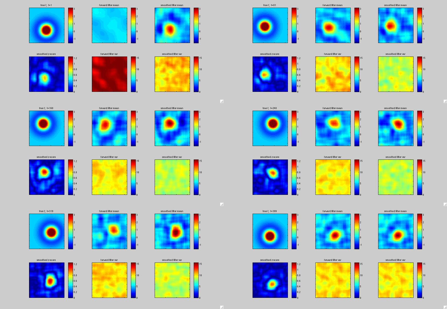
Here are a couple examples.

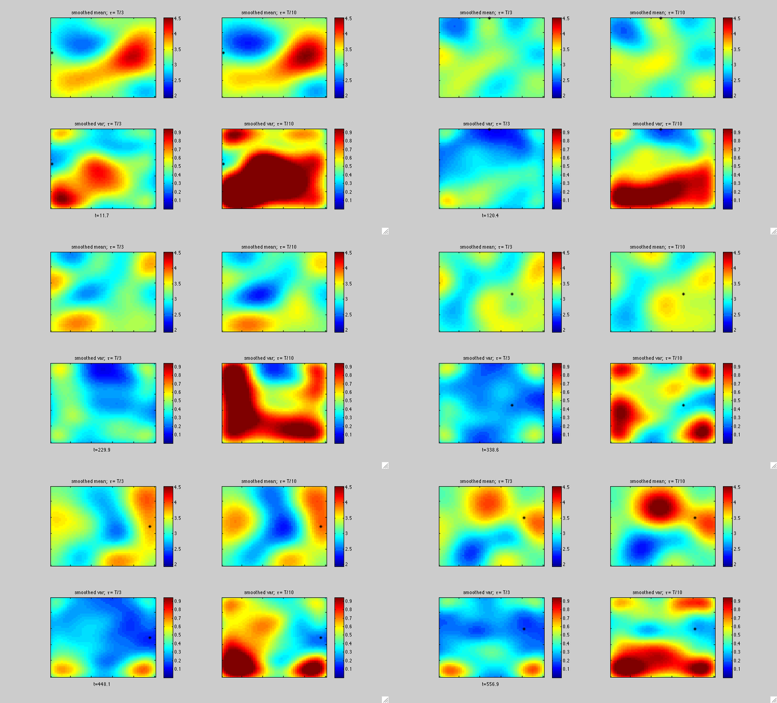
In this first example above, the black dot represents the two-dimensional position x(t) of a mouse wandering around its cage. The position of the mouse was recorded simultaneously with the activity of neurons in the hippocampal formation by Pablo Jercog, who graciously shared this data with us. See Kentros et al 2004 or Muzzio et al 2009 for further details on experimental methods. We applied our filtering methods to estimate the place field f[x,t] of a single neuron as a function of two-dimensional position x and time t: as in the simulated one-dimensional example discussed in the paper, f[x,t] represents the expected firing rate as a function of position x and time t, and is therefore explicitly allowed to change as a function of time. The neuron's observed output at time t, y(t), is represented as y(t)=f[x(t),t]+e(t), where e(t) is a random noise source. The top panels display the fast Kalman filter-smoother output at time t given the observations y(1),...,y(T) at the positions x(1),...,x(T), where T is the length of the experiment (about 500 seconds here), while the bottom panels display the posterior marginal variance (the posterior uncertainty about f[x,t]).

In more detail, we downsampled the position and neural firing rate data to .66 Hz. The spike count in each timebin was transformed to obtain the observation y(t); we applied a standard Anscombe transformation to stabilize the variance of y(t). Under the assumption that the spike counts have approximately Poisson noise, this transformation implies that the variance of the output noise e(t) is of order one. We also fixed the dynamics noise covariance so that the prior equilibrium marginal variance of f was on the order 10, in the units shown in the colorbars above; this is a fairly uninformative prior. This left us with just one free hyperparameter tau (obtained from the dynamics matrix, which was proportional to the identity, as in the examples discussed in the paper). We tried tau=T/3 (left panels) and tau=T/10 (right panels), to get a sense of of the dependence of the estimate on tau. In all cases, we used a Gaussian model for e(t), for simplicity. The place field was modeled as a weighted sum of 400 equally-spaced, isotropic Gaussian bumps, with a total resolution of 50x50=2500 pixels. Full forward-backward smoothing required a few minutes on a laptop; the effective rank of the posterior covariance minus the equilibrium covariance was on the order of 20-40 throughout the experiment.